Category Archives: Analysis

A uniformly but not normally convergent function series

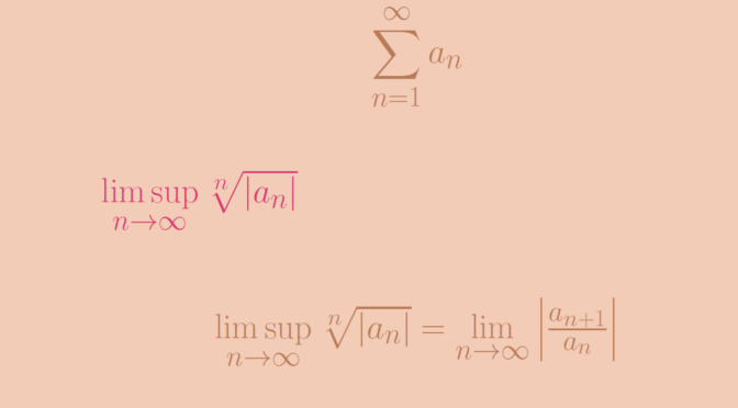
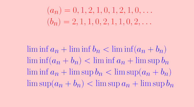
Consider a functions series \(\displaystyle \sum f_n\) of functions defined on a set \(S\) to \(\mathbb R\) or \(\mathbb C\). It is known that if \(\displaystyle \sum f_n\) is normally convergent, then \(\displaystyle \sum f_n\) is uniformly convergent.

The converse is not true and we provide two counterexamples.

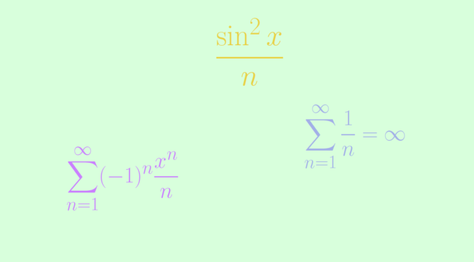
Consider first the sequence of functions \((g_n)\) defined on \(\mathbb R\) by:
\[g_n(x) = \begin{cases}
\frac{\sin^2 x}{n} & \text{for } x \in (n \pi, (n+1) \pi)\\
0 & \text{else}
\end{cases}\] The series \(\displaystyle \sum \Vert g_n \Vert_\infty\) diverges as for all \(n \in \mathbb N\), \(\Vert g_n \Vert_\infty = \frac{1}{n}\) and the harmonic series \(\sum \frac{1}{n}\) diverges. However the series \(\displaystyle \sum g_n\) converges uniformly as for \(x \in \mathbb R\) the sum \(\displaystyle \sum g_n(x)\) is having only one term and \[
\vert R_n(x) \vert = \left\vert \sum_{k=n+1}^\infty g_k(x) \right\vert \le \frac{1}{n+1}\]

For our second example, we consider the sequence of functions \((f_n)\) defined on \([0,1]\) by \(f_n(x) = (-1)^n \frac{x^n}{n}\). For \(x \in [0,1]\) \(\displaystyle \sum (-1)^n \frac{x^n}{n}\) is an alternating series whose absolute value of the terms converge to \(0\) monotonically. According to Leibniz test, \(\displaystyle \sum (-1)^n \frac{x^n}{n}\) is well defined and we can apply the classical inequality \[
\displaystyle \left\vert \sum_{k=1}^\infty (-1)^k \frac{x^k}{k} – \sum_{k=1}^m (-1)^k \frac{x^k}{k} \right\vert \le \frac{x^{m+1}}{m+1} \le \frac{1}{m+1}\] for \(m \ge 1\). Which proves that \(\displaystyle \sum (-1)^n \frac{x^n}{n}\) converges uniformly on \([0,1]\).

However the convergence is not normal as \(\sup\limits_{x \in [0,1]} \frac{x^n}{n} = \frac{1}{n}\).

Root test

The root test is a test for the convergence of a series \[
\sum_{n=1}^\infty a_n \] where each term is a real or complex number. The root test was developed first by Augustin-Louis Cauchy.

We denote \[l = \limsup\limits_{n \to \infty} \sqrt[n]{\vert a_n \vert}.\] \(l\) is a non-negative real number or is possibly equal to \(\infty\). The root test states that:

  • if \(l < 1\) then the series converges absolutely;
  • if \(l > 1\) then the series diverges.

The root test is inconclusive when \(l = 1\).

A case where \(l=1\) and the series diverges

The harmonic series \(\displaystyle \sum_{n=1}^\infty \frac{1}{n}\) is divergent. However \[\sqrt[n]{\frac{1}{n}} = \frac{1}{n^{\frac{1}{n}}}=e^{- \frac{1}{n} \ln n} \] and \(\limsup\limits_{n \to \infty} \sqrt[n]{\frac{1}{n}} = 1\) as \(\lim\limits_{n \to \infty} \frac{\ln n}{n} = 0\).

A case where \(l=1\) and the series converges

Consider the series \(\displaystyle \sum_{n=1}^\infty \frac{1}{n^2}\). We have \[\sqrt[n]{\frac{1}{n^2}} = \frac{1}{n^{\frac{2}{n}}}=e^{- \frac{2}{n} \ln n} \] Therefore \(\limsup\limits_{n \to \infty} \sqrt[n]{\frac{1}{n^2}} = 1\), while the series \(\displaystyle \sum_{n=1}^\infty \frac{1}{n^2}\) is convergent as we have seen in the ratio test article. Continue reading Root test

Ratio test

The ratio test is a test for the convergence of a series \[
\sum_{n=1}^\infty a_n \] where each term is a real or complex number and is nonzero when \(n\) is large. The test is sometimes known as d’Alembert’s ratio test.

Suppose that \[\lim\limits_{n \to \infty} \left\vert \frac{a_{n+1}}{a_n} \right\vert = l\] The ratio test states that:

  • if \(l < 1\) then the series converges absolutely;
  • if \(l > 1\) then the series diverges.

What if \(l = 1\)? One cannot conclude in that case.

Cases where \(l=1\) and the series diverges

Consider the harmonic series \(\displaystyle \sum_{n=1}^\infty \frac{1}{n}\). We have \(\lim\limits_{n \to \infty} \frac{n+1}{n} = 1\). It is well know that the harmonic series diverges. Recall that one proof uses the Cauchy’s convergence test based for \(k \ge 1\) on the inequalities: \[
\sum_{n=2^k+1}^{2^{k+1}} \frac{1}{n} \ge \sum_{n=2^k+1}^{2^{k+1}} \frac{1}{2^{k+1}} = \frac{2^{k+1}-2^k}{2^{k+1}} \ge \frac{1}{2}\]

An even simpler case is the series \(\displaystyle \sum_{n=1}^\infty 1\).

Cases where \(l=1\) and the series converges

We also have \(\lim\limits_{n \to \infty} \left\vert \frac{a_{n+1}}{a_n} \right\vert = 1\) for the infinite series \(\displaystyle \sum_{n=1}^\infty \frac{1}{n^2}\). The series is however convergent as for \(n \ge 1\) we have:\[
0 \le \frac{1}{(n+1)^2} \le \frac{1}{n(n+1)} = \frac{1}{n} – \frac{1}{n+1}\] and the series \(\displaystyle \sum_{n=1}^\infty \left(\frac{1}{n} – \frac{1}{n+1} \right)\) obviously converges.

Another example is the alternating series \(\displaystyle \sum_{n=1}^\infty \frac{(-1)^n}{n}\).

A continuous function with divergent Fourier series

It is known that for a piecewise continuously differentiable function \(f\), the Fourier series of \(f\) converges at all \(x \in \mathbb R\) to \(\frac{f(x^-)+f(x^+)}{2}\).

We describe Fejér example of a continuous function with divergent Fourier series. Fejér example is the even, \((2 \pi)\)-periodic function \(f\) defined on \([0,\pi]\) by: \[
f(x) = \sum_{p=1}^\infty \frac{1}{p^2} \sin \left[ (2^{p^3} + 1) \frac{x}{2} \right]\]
According to Weierstrass M-test, \(f\) is continuous. We denote \(f\) Fourier series by \[
\frac{1}{2} a_0 + (a_1 \cos x + b_1 \sin x) + \dots + (a_n \cos nx + b_n \sin nx) + \dots.\]

As \(f\) is even, the \(b_n\) are all vanishing. If we denote for all \(m \in \mathbb N\):\[
\lambda_{n,m}=\int_0^{\pi} \sin \left[ (2m + 1) \frac{t}{2} \right] \cos nt \ dt \text{ and } \sigma_{n,m} = \sum_{k=0}^n \lambda_{k,m},\]
we have:\[
\begin{aligned}
a_n &=\frac{1}{\pi} \int_{-\pi}^{\pi} f(t) \cos nt \ dt= \frac{2}{\pi} \int_0^{\pi} f(t) \cos nt \ dt\\
&= \frac{2}{\pi} \int_0^{\pi} \left(\sum_{p=1}^\infty \frac{1}{p^2} \sin \left[ (2^{p^3} + 1) \frac{x}{2} \right]\right) \cos nt \ dt\\
&=\frac{2}{\pi} \sum_{p=1}^\infty \frac{1}{p^2} \int_0^{\pi} \sin \left[ (2^{p^3} + 1) \frac{x}{2} \right] \cos nt \ dt\\
&=\frac{2}{\pi} \sum_{p=1}^\infty \frac{1}{p^2} \lambda_{n,2^{p^3-1}}
\end{aligned}\] One can switch the \(\int\) and \(\sum\) signs as the series is normally convergent.

We now introduce for all \(n \in \mathbb N\):\[
S_n = \frac{\pi}{2} \sum_{k=0}^n a_k = \sum_{p=1}^\infty \sum_{k=0}^n \frac{1}{p^2} \lambda_{k,2^{p^3-1}}
=\sum_{p=1}^\infty \frac{1}{p^2} \sigma_{n,2^{p^3-1}}\]

We will prove below that for all \(n,m \in \mathbb N\) we have \(\sigma_{m,m} \ge \frac{1}{2} \ln m\) and \(\sigma_{n,m} \ge 0\). Assuming those inequalities for now, we get:\[
S_{2^{p^3-1}} \ge \frac{1}{p^2} \sigma_{2^{p^3-1},2^{p^3-1}} \ge \frac{1}{2p^2} \ln(2^{p^3-1}) = \frac{p^3-1}{2p^2} \ln 2\]
As the right hand side diverges to \(\infty\), we can conclude that \((S_n)\) diverges and consequently that the Fourier series of \(f\) diverges at \(0\). Continue reading A continuous function with divergent Fourier series

Radius of convergence of power series

We look here at the radius of convergence of the sum and product of power series.

Let’s recall that for a power series \(\displaystyle \sum_{n=0}^\infty a_n x^n\) where \(0\) is not the only convergence point, the radius of convergence is the unique real \(0 < R \le \infty\) such that the series converges whenever \(\vert x \vert < R\) and diverges whenever \(\vert x \vert > R\).

Given two power series with radii of convergence \(R_1\) and \(R_2\), i.e.
\begin{align*}
\displaystyle f_1(x) = \sum_{n=0}^\infty a_n x^n, \ \vert x \vert < R_1 \\ \displaystyle f_2(x) = \sum_{n=0}^\infty b_n x^n, \ \vert x \vert < R_2 \end{align*} The sum of the power series \begin{align*} \displaystyle f_1(x) + f_2(x) &= \sum_{n=0}^\infty a_n x^n + \sum_{n=0}^\infty b_n x^n \\ &=\sum_{n=0}^\infty (a_n + b_n) x^n \end{align*} and its Cauchy product:
\begin{align*}
\displaystyle f_1(x) \cdot f_2(x) &= \left(\sum_{n=0}^\infty a_n x^n\right) \cdot \left(\sum_{n=0}^\infty b_n x^n \right) \\
&=\sum_{n=0}^\infty \left( \sum_{l=0}^n a_l b_{n-l}\right) x^n
\end{align*}
both have radii of convergence greater than or equal to \(\min \{R_1,R_2\}\).

The radii can indeed be greater than \(\min \{R_1,R_2\}\). Let’s give examples.
Continue reading Radius of convergence of power series

Counterexample around Morera’s theorem

Let’s recall Morera’s theorem.

Morera’s theorem
Suppose that \(f\) is a continuous complex-valued function in a connected open set \(\Omega \subset \mathbb C\) such that
\[\int_{\partial \Delta} f(z) \ dz = 0\] for every closed triangle \(\Delta \subset \Omega \setminus \{p\}\) where \(p \in \Omega\). Then \(f\) is holomorphic in \(\Omega\).

Does the conclusion of Morera’s theorem still hold if \(f\) is supposed to be continuous only in \(\Omega \setminus \{p\}\)? The answer is negative and we provide a counterexample.

Let \(\Omega\) be the entire complex plane, \(f\) defined as follows
\[f(z)=\begin{cases}
\frac{1}{z^2} & \text{if } z \neq 0\\
0 & \text{otherwise}
\end{cases}\] and \(p\) the origin.

For \(a,b \in \Omega \setminus \{0\}\) we have
\[\begin{aligned}
\int_{[a,b]} f(z) \ dz &= \int_{[a,b]} \frac{dz}{z^2}\\
&= \int_0^1 \frac{b-a}{[a+t(b-a)]^2} \ dt\\
&=\left[ -\frac{1}{a+t(b-a)} \right]_0^1 = \frac{1}{a} – \frac{1}{b}
\end{aligned}\]

Hence for a triangle \(\Delta\) with vertices at \(a,b ,c \in \Omega \setminus \{0\}\):
\[\int_{\partial \Delta} f(z) \ dz = \left( \frac{1}{a} – \frac{1}{b} \right) + \left( \frac{1}{b} – \frac{1}{c} \right) + \left( \frac{1}{c} – \frac{1}{a} \right)=0\]

However, \(f\) is not holomorphic in \(\Omega\) as it is even not continuous at \(0\).

Continuity versus uniform continuity

We consider real-valued functions.

A real-valued function \(f : I \to \mathbb R\) (where \(I \subseteq\) is an interval) is continuous at \(x_0 \in I\) when: \[(\forall \epsilon > 0) (\exists \delta > 0)(\forall x \in I)(\vert x- x_0 \vert \le \delta \Rightarrow \vert f(x)- f(x_0) \vert \le \epsilon).\] When \(f\) is continuous at all \(x \in I\), we say that \(f\) is continuous on \(I\).

\(f : I \to \mathbb R\) is said to be uniform continuity on \(I\) if \[(\forall \epsilon > 0) (\exists \delta > 0)(\forall x,y \in I)(\vert x- y \vert \le \delta \Rightarrow \vert f(x)- f(y) \vert \le \epsilon).\]

Obviously, a function which is uniform continuous on \(I\) is continuous on \(I\). Is the converse true? The answer is negative.

An (unbounded) continuous function which is not uniform continuous

The map \[
\begin{array}{l|rcl}
f : & \mathbb R & \longrightarrow & \mathbb R \\
& x & \longmapsto & x^2 \end{array}\] is continuous. Let’s prove that it is not uniform continuous. For \(0 < x < y\) we have \[\vert f(x)-f(y) \vert = y^2-x^2 = (y-x)(y+x) \ge 2x (y-x)\] Hence for \(y-x= \delta >0\) and \(x = \frac{1}{\delta}\) we get
\[\vert f(x) -f(y) \vert \ge 2x (y-x) =2 > 1\] which means that the definition of uniform continuity is not fulfilled for \(\epsilon = 1\).

For this example, the function is unbounded as \(\lim\limits_{x \to \infty} x^2 = \infty\). Continue reading Continuity versus uniform continuity

Continuity under the integral sign

We consider here a measure space \((\Omega, \mathcal A, \mu)\) and \(T \subset \mathbb R\) a topological subspace. For a map \(f : T \times \Omega \to \mathbb R\) such that for all \(t \in T\) the map \[
\begin{array}{l|rcl}
f(t, \cdot) : & \Omega & \longrightarrow & \mathbb R \\
& \omega & \longmapsto & f(t,\omega) \end{array}
\] is integrable, one can define the function \[
\begin{array}{l|rcl}
F : & T & \longrightarrow & \mathbb R \\
& t & \longmapsto & \int_\Omega f(t,\omega) \ d\mu(\omega) \end{array}
\]

Following theorem is well known (and can be proven using dominated convergence theorem):

THEOREM for an adherent point \(x \in T\), if

  • \(\forall \omega \in \Omega \lim\limits_{t \to x} f(t,\omega) = \varphi(\omega)\)
  • There exists a map \(g : \Omega \to \mathbb R\) such that \(\forall t \in T, \, \forall \omega \in \Omega, \ \vert f(t,\omega) \vert \le g(\omega)\)

then \(\varphi\) is integrable and \[
\lim\limits_{t \to x} F(t) = \int_\Omega \varphi(\omega) \ d\mu(\omega)\]
In other words, one can switch \(\lim\) and \(\int\) signs.

We provide here a counterexample showing that the conclusion of the theorem might not hold if \(f\) is not bounded by a function \(g\) as supposed in the premises of the theorem. Continue reading Continuity under the integral sign

A trigonometric series that is not a Fourier series (Lebesgue-integration)

We already provided here an example of a trigonometric series that is not the Fourier series of a Riemann-integrable function (namely the function \(\displaystyle x \mapsto \sum_{n=1}^\infty \frac{\sin nx}{\sqrt n}\)).

Applying an Abel-transformation (like mentioned in the link above), one can see that the function \[f(x)=\sum_{n=2}^\infty \frac{\sin nx}{\ln n}\] is everywhere convergent. We now prove that \(f\) cannot be the Fourier series of a Lebesgue-integrable function. The proof is based on the fact that for a \(2 \pi\)-periodic function \(g\), Lebesgue-integrable on \([0,2 \pi]\), the sum \[\sum_{n=1}^\infty \frac{c_n-c_{-n}}{n}\] is convergent where \((c_n)_{n \in \mathbb Z}\) are the complex Fourier coefficients of \(g\): \[c_n = \frac{1}{2 \pi} \int_0^{2 \pi} g(t)e^{-ikt} \ dt.\] As the series \(\displaystyle \sum_{n=2}^\infty \frac{1}{n \ln n}\) is divergent, we will be able to conclude that the sequence defined by \[\gamma_0=\gamma_1=\gamma_{-1} = 0, \, \gamma_n=- \gamma_{-n} = \frac{1}{\ln n} \ (n \ge 2)\] cannot be the Fourier coefficients of a Lebesgue-integrable function, hence that \(f\) is not the Fourier series of any Lebesgue-integrable function. Continue reading A trigonometric series that is not a Fourier series (Lebesgue-integration)

Playing with liminf and limsup

Let’s consider real sequences \((a_n)_{n \in \mathbb N}\) and \((b_n)_{n \in \mathbb N}\). We look at inequalities involving limit superior and limit inferior of those sequences. Following inequalities hold:
\[\begin{aligned}
& \liminf a_n + \liminf b_n \le \liminf (a_n+b_n)\\
& \liminf (a_n+b_n) \le \liminf a_n + \limsup b_n\\
& \liminf a_n + \limsup b_n \le \limsup (a_n+b_n)\\
& \limsup (a_n+b_n) \le \limsup a_n + \limsup b_n
\end{aligned}\] Let’s prove for example the first inequality, reminding first that \[
\liminf\limits_{n \to \infty} a_n = \lim\limits_{n \to \infty} \left(\inf\limits_{m \ge n} a_m \right).\] For \(n \in \mathbb N\), we have for all \(m \ge n\) \[\inf\limits_{k \ge n} a_k + \inf\limits_{k \ge n} b_k \le a_m + b_m\] hence \[\inf\limits_{k \ge n} a_k + \inf\limits_{k \ge n} b_k \le \inf\limits_{k \ge n} \left(a_k+b_k \right)\] As the sequences \((\inf\limits_{k \ge n} a_k)_{n \in \mathbb N}\) and \((\inf\limits_{k \ge n} b_k)_{n \in \mathbb N}\) are non-increasing we get for all \(n \in \mathbb N\), \[\liminf a_n + \liminf b_n \le \inf\limits_{m \ge n} \left(a_m+b_m \right)\] which leads finally to the desired inequality \[\liminf a_n + \liminf b_n \le \liminf (a_n+b_n).\] Continue reading Playing with liminf and limsup