A trigonometric series that is not a Fourier series (Riemann-integration)

We’re looking here at convergent trigonometric series like \[f(x) = a_0 + \sum_{k=1}^\infty (a_n \cos nx + b_n \sin nx)\] which are convergent but are not Fourier series. Which means that the terms \(a_n\) and \(b_n\) cannot be written\[
\begin{array}{ll}
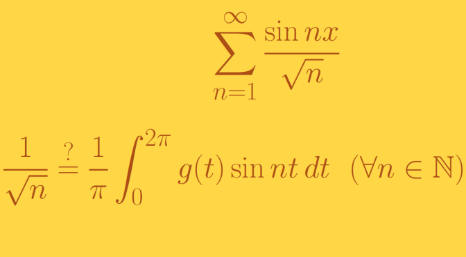
a_n = \frac{1}{\pi} \int_0^{2 \pi} g(t) \cos nt \, dt & (n= 0, 1, \dots) \\
b_n = \frac{1}{\pi} \int_0^{2 \pi} g(t) \sin nt \, dt & (n= 1, 2, \dots)
\end{array}\] where \(g\) is any integrable function.

This raises the question of the type of integral used. We cover here an example based on Riemann integral. I’ll cover a Lebesgue integral example later on.

We prove here that the function \[
f(x)= \sum_{n=1}^\infty \frac{\sin nx}{\sqrt{n}}\] is a convergent trigonometric series but is not a Fourier series. Continue reading A trigonometric series that is not a Fourier series (Riemann-integration)

Counterexamples around cardinality (part 1)

In mathematics, the cardinality of a set is a measure of the “number of elements of the set”. We denote by \(|A|\) the cardinality of the set \(A\). We say that \(A\) and \(B\) have the same cardinality if there exists a bijection from \(A\) onto \(B\). Such sets said to be equinumerous.

The finite sets satisfy the property that if \(A \subset B\) and \(A\) and \(B\) have the same cardinality then \(A=B\). For example take \(A=\{2,5,42\}\). If \(A \subset B\) and \(B\) has more elements than \(A\), a bijection \(f\) from \(A\) to \(B\) cannot exist as an element in \(B \setminus \{f(2),f(5),f(42)\}\) won’t have an inverse image under \(f\).

This becomes false for infinite sets. Let’s give some examples.

Proper subsets of \(\mathbb N\) equinumerous to \(\mathbb N\)

The set \(A\) of the positive even integers is strictly included in \(\mathbb N\): there exist odd positive integers! However, \(A\) is equinumerous to \(\mathbb N\). The map \(f : n \to 2n\) is a bijection from \(A\) onto \(\mathbb N\).

For our second example, consider the set \(\mathbb P\) of prime numbers. We recall that \(\mathbb P\) is infinite. The proof is quite simple by contradiction. Suppose that there is only a finite number \(\{p_1, \dots, p_n\}\) of prime numbers and consider the number \(N = p_1 p_2 \cdots p_n + 1\). As a consequence of the fundamental theorem of arithmetic, a prime \(q\) divides \(N\). However \(q \notin \{p_1, \dots, p_n\}\) as this would imply \(q\) divides \(1\). From there, we can define by induction a bijection from \(\mathbb N\) onto \(\mathbb P\) by defining \[f(n)=\begin{cases}
2 & \text{for } n=1\\
\min (\mathbb P \setminus \{p_1, \dots, p_n\}) & \text{else }
\end{cases}\] Continue reading Counterexamples around cardinality (part 1)

Infinite rings and fields with positive characteristic

Familiar to us are infinite fields whose characteristic is equal to zero like \(\mathbb Z, \mathbb Q, \mathbb R\) or the field of constructible numbers.

We’re also familiar with rings having infinite number of elements and zero for characteristic like:

  • The rings of polynomials \(\mathbb Z[X], \mathbb Q[X], \mathbb R[X]\).
  • The rings of matrices \(\mathcal{M}_2(\mathbb R)\).
  • Or the ring of real continuous functions defined on \(\mathbb R\).

We also know rings or fields like integers modulo \(n\) (with \(n \ge 2\)) \(\mathbb Z_n\) or the finite field \(\mathbb F_q\) with \(q=p^r\) elements where \(p\) is a prime.

We provide below examples of infinite rings or fields with positive characteristic.

Infinite rings with positive characteristic

Consider the ring \(\mathbb Z_n[X]\) of polynomials in one variable \(X\) with coefficients in \(\mathbb Z_n\) for \(n \ge 2\) integer. It is an infinite ring since \(\mathbb X^m \in \mathbb{Z}_n[X]\) for all positive integers \(m\), and \(X^r \neq X^s\) for \(r \neq s\). But the characteristic of \(\mathbb Z_n[X]\) is clearly \(n\).

Another example is based on product of rings. If \(I\) is an index set and \((R_i)_{i \in I}\) a family of rings, one can define the product ring \(\displaystyle \prod_{i \in I} R_i\). The operations are defined the natural way with \((a_i)_{i \in I} + (b_i)_{i \in I} = (a_i+b_i)_{i \in I}\) and \((a_i)_{i \in I} \cdot (b_i)_{i \in I} = (a_i \cdot b_i)_{i \in I}\). Fixing \(n \ge 2\) integer and taking \(I = \mathbb N\), \(R_i = \mathbb Z_n\) for all \(i \in I\) we get the ring \(\displaystyle R = \prod_{k \in \mathbb N} \mathbb Z_n\). \(R\) multiplicative identity is the sequence with all terms equal to \(1\). The characteristic of \(R\) is \(n\) and \(R\) is obviously infinite. Continue reading Infinite rings and fields with positive characteristic

Playing with images and inverse images

We’re looking here to relational expressions involving image and inverse image.

We consider a function \(f : X \to Y\) from the set \(X\) to the set \(Y\). If \(x\) is a member of \(X\), \(f(x)\) is the image of \(x\) under \(f\).
The image of a subset \(A \subset X\) under \(f\) is the subset (of \(Y\)) \[f(A)\stackrel{def}{=} \{f(x) : x \in A\}.\]

The inverse image of a subset \(B \subset Y\) is the subset of \(A\) \[f^{-1}(B)\stackrel{def}{=} \{x \in X : f(x) \in B\}.\] Important to understand is that here, \(f^{-1}\) is not the inverse function of \(f\).

We now look at relational expressions involving the image and the inverse image under \(f\).

Inverse images with unions and intersections

Following relations hold:
\[\begin{array}{c}
f^{-1}(B_1 \cup B_2) = f^{-1}(B_1) \cup f^{-1}(B_2)\\
f^{-1}(B_1 \cap B_2) = f^{-1}(B_1) \cap f^{-1}(B_2)
\end{array}\] Let’s prove the first equality as an example. We have \(x \in f^{-1}(B_1 \cup B_2)\) if and only if \(f(x) \in B_1 \cup B_2\) if and only if \(f(x) \in B_1\) or \(f(x) \in B_2\) which means exactly \(x \in f^{-1}(B_1) \cup f^{-1}(B_2)\). Continue reading Playing with images and inverse images

Counterexamples around balls in metric spaces

Let’s play with balls in a metric space \((M,d)\). We denote by

  • \(B_r(p) = \{x \in M : d(x,p) < r\}\) the open ball.
  • \(B_r[p] = \{x \in M : d(x,p) \le r\}\) the closed ball.

A ball of radius \(r\) included in a ball of radius \(r^\prime < r\)

We take for \(M\) the space \(\{0\} \cup [2, \infty)\) equipped with the standard metric distance \(d(x,y)=\vert x – y \vert\).

We have \(B_4(0) = \{0\} \cup [2, 4)\) while \(B_3(2) = \{0\} \cup [2, 5)\). Despite having a strictly smaller radius, the ball \(B_3(2)\) strictly contains the ball \(B_4(0)\).

The phenomenon cannot happen in a normed vector space \((M, \Vert \cdot \Vert)\). For the proof, take two open balls \(B_r(p),B_{r^\prime}(p^\prime) \subset M\), \(0 < r^\prime < r\) and suppose that \(p \in B_{r^\prime}(p^\prime)\). If \(p=p^\prime\) and \(q \in B_{r^\prime}(p^\prime) \setminus \{p^\prime\}\) then \(p + \frac{\frac{r+r^\prime}{2} }{\Vert p q \Vert} p q \in B_r(p) \setminus B_{r^\prime}(p^\prime) \). And if \(p \neq p^\prime\), \(p \in B_{r^\prime}(p^\prime)\) then \(p^\prime + \frac{\frac{r+r^\prime}{2} }{\Vert p^\prime p \Vert} p^\prime p \in B_r(p) \setminus B_{r^\prime}(p^\prime) \).

An open ball \(B_r(p)\) whose closure is not equal to the closed ball \(B_r[p]\)

Here we take for \(M\) a subspace of \(\mathbb R^2\) which is the union of the origin \(\{0\}\) with the unit circle \(S^1\). For the distance, we use the Euclidean norm.
The open unit ball centered at the origin \(B_1(0)\) is reduced to the origin: \(B_1(0) = \{0\}\). Its closure \(\overline{B_1(0)}\) is itself. However the closed ball \(B_1[0]\) is the all space \(\{0\} \cup S^1\).

Again one can prove that for a normed vector space this cannot happen. The closure of an open ball is the closed ball for a normed vector space.

Counterexamples around Dini’s theorem

In this article we look at counterexamples around Dini’s theorem. Let’s recall:

Dini’s theorem: If \(K\) is a compact topological space, and \((f_n)_{n \in \mathbb N}\) is a monotonically decreasing sequence (meaning \(f_{n+1}(x) \le f_n(x)\) for all \(n \in \mathbb N\) and \(x \in K\)) of continuous real-valued functions on \(K\) which converges pointwise to a continuous function \(f\), then the convergence is uniform.

We look at what happens to the conclusion if we drop some of the hypothesis.

Cases if \(K\) is not compact

We take \(K=(0,1)\), which is not closed equipped with the common distance. The sequence \(f_n(x)=x^n\) of continuous functions decreases pointwise to the always vanishing function. But the convergence is not uniform because for all \(n \in \mathbb N\) \[\sup\limits_{x \in (0,1)} x^n = 1\]

The set \(K=\mathbb R\) is closed but unbounded, hence also not compact. The sequence defined by \[f_n(x)=\begin{cases}
0 & \text{for } x < n\\ \frac{x-n}{n} & \text{for } n \le x < 2n\\ 1 & \text{for } x \ge 2n \end{cases}\] is continuous and monotonically decreasing. It converges to \(0\). However, the convergence is not uniform as for all \(n \in \mathbb N\): \(\sup\{f_n(x) : x \in \mathbb R\} =1\). Continue reading Counterexamples around Dini’s theorem

A ring whose characteristic is a prime having a zero divisor

Consider a ring \(R\) whose characteristic is a composite number \(p=ab\) with \(a,b\) integers greater than \(1\). Then \(R\) has a zero divisor as we have \[0=p.1=(a.b).1=(a.1).(b.1).\]

What can we say of a ring \(R\) having zero divisors? It is known that the rings \(\mathbb{Z}/p.\mathbb{Z}\) where \(p\) is a prime are fields and therefore do not have zero divisors. Is this a general fact? That is, does a ring whose characteristic is a prime do not have zero divisors?

The answer is negative and we give below a counterexample.

Let’s consider the field \(\mathbb{F}_p = \mathbb{Z}/p.\mathbb{Z}\) where \(p\) is a prime and the product of rings \(R=\mathbb{F}_p \times \mathbb{F}_p\). One can verify following facts:

  • \(R\) additive identity is equal to \((0,0)\).
  • \(R\) multiplicative identity is equal to \((1,1)\).
  • \(R\) is commutative.
  • The characteristic of \(R\) is equal to \(p\) as for \(n\) integer, we have \(n.(1,1)=(n.1,n.1)\) which is equal to \((0,0)\) if and only if \(p\) divides \(n\).

However, \(R\) does have zero divisors as following identity holds: \[(1,0).(0,1)=(0,0)\]

The Smith Volterra Cantor Set

In Cantor set article, I presented the Cantor set which is a null set having the cardinality of the continuum. I present here a modification of the Cantor set named the Smith-Volterra-Cantor set.

Construction of the Smith-Volterra-Cantor set

The Smith-Volterra-Cantor set (also named SVC set below) \(S\) is a subset of the real segment \(I=[0,1]\). It is built by induction:

  • Starting with \(S_0=I\)
  • \(S_1=[0,\frac{3}{8}] \cup [\frac{5}{8},1]\)
  • If \(S_n\) is a finite disjoint union of segments \(s_n=\cup_k \left[a_k,b_k\right]\), \[S_{n+1}=\bigcup_k \left(\left[a_k,\frac{a_k+b_k}{2}-\frac{1}{2^{2n+3}}\right] \cup \left[\frac{a_k+b_k}{2}+\frac{1}{2^{2n+3}},b_k\right]\right)\]

Continue reading The Smith Volterra Cantor Set

No minimum at the origin but a minimum along all lines

We look here at an example, from the Italian mathematician Giuseppe Peano of a real function \(f\) defined on \(\mathbb{R}^2\). \(f\) is having a local minimum at the origin along all lines passing through the origin, however \(f\) does not have a local minimum at the origin as a function of two variables.

The function \(f\) is defined as follows
\[\begin{array}{l|rcl}
f : & \mathbb{R}^2 & \longrightarrow & \mathbb{R} \\
& (x,y) & \longmapsto & f(x,y)=3x^4-4x^2y+y^2 \end{array}\] One can notice that \(f(x, y) = (y-3x^2)(y-x^2)\). In particular, \(f\) is strictly negative on the open set \(U=\{(x,y) \in \mathbb{R}^2 \ : \ x^2 < y < 3x^2\}\), vanishes on the parabolas \(y=x^2\) and \(y=3 x^2\) and is strictly positive elsewhere. Consider a line \(D\) passing through the origin. If \(D\) is different from the coordinate axes, the equation of \(D\) is \(y = \lambda x\) with \(\lambda > 0\). We have \[f(x, \lambda x)= x^2(\lambda-3x)(\lambda -x).\] For \(x \in (-\infty,\frac{\lambda}{3}) \setminus \{0\}\), \(f(x, \lambda x) > 0\) while \(f(0,0)=0\) which proves that \(f\) has a local minimum at the origin along the line \(D \equiv y – \lambda x=0\). Along the \(x\)-axis, we have \(f(x,0)=3 x^ 4\) which has a minimum at the origin. And finally, \(f\) also has a minimum at the origin along the \(y\)-axis as \(f(0,y)=y^2\).

However, along the parabola \(\mathcal{P} \equiv y = 2 x^2\) we have \(f(x,2 x^2)=-x^4\) which is strictly negative for \(x \neq 0\). As \(\mathcal{P}\) is passing through the origin, \(f\) assumes both positive and negative values in all neighborhood of the origin.

This proves that \(f\) does not have a minimum at \((0,0)\).

Two matrices A and B for which AB and BA have different minimal polynomials

We consider here the algebra of matrices \(\mathcal{M}_n(\mathbb F)\) of dimension \(n \ge 1\) over a field \(\mathbb F\).

It is well known that for \(A,B \in \mathcal{M}_n(\mathbb F)\), the characteristic polynomial \(p_{AB}\) of the product \(AB\) is equal to the one (namely \(p_{BA}\)) of the product of \(BA\). What about the minimal polynomial?

Unlikely for the characteristic polynomials, the minimal polynomial \(\mu_{AB}\) of \(AB\) maybe different to the one of \(BA\).

Consider the two matrices \[
A=\begin{pmatrix}
0 & 1\\
0 & 0\end{pmatrix} \text{, }
B=\begin{pmatrix}
0 & 0\\
0 & 1\end{pmatrix}\] which can be defined whatever the field we consider: \(\mathbb R, \mathbb C\) or even a field of finite characteristic.

One can verify that \[
AB=A=\begin{pmatrix}
0 & 1\\
0 & 0\end{pmatrix} \text{, }
BA=\begin{pmatrix}
0 & 0\\
0 & 0\end{pmatrix}\]

As \(BA\) is the zero matrix, its minimal polynomial is \(\mu_{BA}=X\). Regarding the one of \(AB\), we have \((AB)^2=A^2=0\) hence \(\mu_{AB}\) divides \(X^2\). Moreover \(\mu_{AB}\) cannot be equal to \(X\) as \(AB \neq 0\). Finally \(\mu_{AB}=X^2\) and we verify that \[X^2=\mu_{AB} \neq \mu_{BA}=X.\]

Mathematical exceptions to the rules or intuition