All posts by Jean-Pierre Merx

A discontinuous midpoint convex function

Let’s recall that a real function \(f: \mathbb R \to \mathbb R\) is called convex if for all \(x, y \in \mathbb R\) and \(\lambda \in [0,1]\) we have \[
f((1- \lambda) x + \lambda y) \le (1- \lambda) f(x) + \lambda f(y)\] \(f\) is called midpoint convex if for all \(x, y \in \mathbb R\) \[
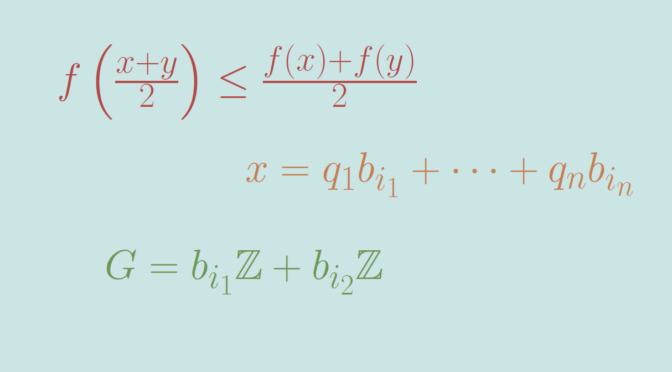
f \left(\frac{x+y}{2}\right) \le \frac{f(x)+f(y)}{2}\] One can prove that a continuous midpoint convex function is convex. Sierpinski proved the stronger theorem, that a real-valued Lebesgue measurable function that is midpoint convex will be convex.

Can one find a discontinuous midpoint convex function? The answer is positive but requires the Axiom of Choice. Why? Because Robert M. Solovay constructed a model of Zermelo-Fraenkel set theory (ZF), exclusive of the axiom of choice where all functions are Lebesgue measurable. Hence convex according to Sierpinski theorem. And one knows that convex functions defined on \(\mathbb R\) are continuous.

Referring to my previous article on the existence of discontinuous additive map, let’s use a Hamel basis \(\mathcal B = (b_i)_{i \in I}\) of \(\mathbb R\) considered as a vector space on \(\mathbb Q\). Take \(i_1 \in I\), define \(f(i_1)=1\) and \(f(i)=0\) for \(i \in I\setminus \{i_1\}\) and extend \(f\) linearly on \(\mathbb R\). \(f\) is midpoint convex as it is linear. As the image of \(\mathbb R\) under \(f\) is \(\mathbb Q\), \(f\) is discontinuous as explained in the discontinuous additive map counterexample.

Moreover, \(f\) is unbounded on all open real subsets. By linearity, it is sufficient to prove that \(f\) is unbounded around \(0\). Let’s consider \(i_1 \neq i_2 \in I\). \(G= b_{i_1} \mathbb Z + b_{i_2} \mathbb Z\) is a proper subgroup of the additive \(\mathbb R\) group. Hence \(G\) is either dense of discrete. It cannot be discrete as the set of vectors \(\{b_1,b_2\}\) is linearly independent. Hence \(G\) is dense in \(\mathbb R\). Therefore, one can find a non vanishing sequence \((x_n)_{n \in \mathbb N}=(q_n^1 b_{i_1} + q_n^2 b_{i_2})_{n \in \mathbb N}\) (with \((q_n^1,q_n^2) \in \mathbb Q^2\) for all \(n \in \mathbb N\)) converging to \(0\). As \(\{b_1,b_2\}\) is linearly independent, this implies \(\vert q_n^1 \vert, \vert q_n^2 \vert \underset{n\to+\infty}{\longrightarrow} \infty\) and therefore \[
\lim\limits_{n \to \infty} \vert f(x_n) \vert = \lim\limits_{n \to \infty} \vert f(q_n^1 b_{i_1} + q_n^2 b_{i_2}) \vert = \lim\limits_{n \to \infty} \vert q_n^1 \vert = \infty.\]

A discontinuous additive map

A function \(f\) defined on \(\mathbb R\) into \(\mathbb R\) is said to be additive if and only if for all \(x, y \in \mathbb R\)
\[f(x+y) = f(x) + f(y).\] If \(f\) is supposed to be continuous at zero, \(f\) must have the form \(f(x)=cx\) where \(c=f(1)\). This can be shown using following steps:

  • \(f(0) = 0\) as \(f(0) = f(0+0)= f(0)+f(0)\).
  • For \(q \in \mathbb N\) \(f(1)=f(q \cdot \frac{1}{q})=q f(\frac{1}{q})\). Hence \(f(\frac{1}{q}) = \frac{f(1)}{q}\). Then for \(p,q \in \mathbb N\), \(f(\frac{p}{q}) = p f(\frac{1}{q})= f(1) \frac{p}{q}\).
  • As \(f(-x) = -f(x)\) for all \(x \in\mathbb R\), we get that for all rational number \(\frac{p}{q} \in \mathbb Q\), \(f(\frac{p}{q})=f(1)\frac{p}{q}\).
  • The equality \(f(x+y) = f(x) + f(y)\) implies that \(f\) is continuous on \(\mathbb R\) if it is continuous at \(0\).
  • We can finally conclude to \(f(x)=cx\) for all real \(x \in \mathbb R\) as the rational numbers are dense in \(\mathbb R\).

We’ll use a Hamel basis to construct a discontinuous linear function. The set \(\mathbb R\) can be endowed with a vector space structure over \(\mathbb Q\) using the standard addition and the multiplication by a rational for the scalar multiplication.

Using the axiom of choice, one can find a (Hamel) basis \(\mathcal B = (b_i)_{i \in I}\) of \(\mathbb R\) over \(\mathbb Q\). That means that every real number \(x\) is a unique linear combination of elements of \(\mathcal B\): \[
x= q_1 b_{i_1} + \dots + q_n b_{i_n}\] with rational coefficients \(q_1, \dots, q_n\). The function \(f\) is then defined as \[
f(x) = q_1 + \dots + q_n.\] The linearity of \(f\) follows from its definition. \(f\) is not continuous as it only takes rational values which are not all equal. And one knows that the image of \(\mathbb R\) under a continuous map is an interval.

Existence of a continuous function with divergent Fourier series

In that article, I provided an example of a continuous function with divergent Fourier series. We prove here the existence of such a function using Banach-Steinhaus theorem, also called uniform boundedness principle.

Theorem (Uniform Boundedness Theorem) Let \((X, \Vert \cdot \Vert_X)\) be a Banach space and \((Y, \Vert \cdot \Vert_Y)\) be a normed vector space. Suppose that \(F\) is a set of continuous linear operators from \(X\) to \(Y\). If for all \(x \in X\) one has \[
\sup\limits_{T \in F} \Vert T(x) \Vert_Y \lt \infty\] then \[
\sup\limits_{T \in F, \ \Vert x \Vert = 1} \Vert T(x) \Vert_Y \lt \infty\]

Let’s take for \(X\) the vector space \(\mathcal C_{2 \pi}\) of continuous functions from \(\mathbb R\) to \(\mathbb C\) which are periodic with period \(2 \pi\) endowed with the norm \(\Vert f \Vert_\infty = \sup\limits_{- \pi \le t \le \pi} \vert f(t) \vert\). \((\mathcal C_{2 \pi}, \Vert \cdot \Vert_\infty)\) is a Banach space. For the vector space \(Y\), we take the complex numbers \(\mathbb C\) endowed with the modulus.

For \(n \in \mathbb N\), the map \[
\begin{array}{l|rcl}
\ell_n : & \mathcal C_{2 \pi} & \longrightarrow & \mathbb C \\
& f & \longmapsto & \displaystyle \sum_{p=-n}^n c_p(f) \end{array}\] is a linear operator, where for \(p \in \mathbb Z\), \(c_p(f)\) denotes the complex Fourier coefficient \[
c_p(f) = \frac{1}{2 \pi} \int_{- \pi}^{\pi} f(t) e^{-i p t} \ dt\]

We now prove that
\begin{align*}
\Lambda_n &= \sup\limits_{f \in \mathcal C_{2 \pi}, \Vert f \Vert_\infty=1} \vert \ell_n(f) \vert\\
&= \frac{1}{2 \pi} \int_{- \pi}^{\pi} \left\vert \frac{\sin (2n+1)\frac{t}{2}}{\sin \frac{t}{2}} \right\vert \ dt = \frac{1}{2 \pi} \int_{- \pi}^{\pi} \left\vert h_n(t) \right\vert \ dt,
\end{align*} where one can notice that the function \[
\begin{array}{l|rcll}
h_n : & [- \pi, \pi] & \longrightarrow & \mathbb C \\
& t & \longmapsto & \frac{\sin (2n+1)\frac{t}{2}}{\sin \frac{t}{2}} &\text{for } t \neq 0\\
& 0 & \longmapsto & 2n+1
\end{array}\] is continuous.
Continue reading Existence of a continuous function with divergent Fourier series

A positive smooth function with all derivatives vanishing at zero

Let’s consider the set \(\mathcal C^\infty(\mathbb R)\) of real smooth functions, i.e. functions that have derivatives of all orders on \(\mathbb R\).

Does a positive function \(f \in \mathcal C^\infty(\mathbb R)\) with all derivatives vanishing at zero exists?

Such a map \(f\) cannot be expandable in power series around zero, as it would vanish in a neighborhood of zero. However, the answer to our question is positive and we’ll prove that \[
f(x) = \left\{\begin{array}{lll}
e^{-\frac{1}{x^2}} &\text{if} &x \neq 0\\
0 &\text{if} &x = 0 \end{array}\right. \] provides an example.

\(f\) is well defined and positive for \(x \neq 0\). As \(\lim\limits_{x \to 0} -\frac{1}{x^2} = -\infty\), we get \(\lim\limits_{x \to 0} f(x) = 0\) proving that \(f\) is continuous on \(\mathbb R\). Let’s prove by induction that for \(x \neq 0\) and \(n \in \mathbb N\), \(f^{(n)}(x)\) can be written as \[
f^{(n)}(x) = \frac{P_n(x)}{x^{3n}}e^{-\frac{1}{x^2}}\] where \(P_n\) is a polynomial function. The statement is satisfied for \(n = 1\) as \(f^\prime(x) = \frac{2}{x^3}e^{-\frac{1}{x^2}}\). Suppose that the statement is true for \(n\) then \[
f^{(n+1)}(x)=\left[\frac{P_n^\prime(x)}{x^{3n}} – \frac{3n P_n(x)}{x^{3n+1}}+\frac{2 P_n(x)}{x^{3n+3}}\right] e^{-\frac{1}{x^2}}\] hence the statement is also true for \(n+1\) by taking \(P_{n+1}(x)=
x^3 P_n^\prime(x) – 3n x^2 P_n(x) + 2 P_n(x)\). Which concludes our induction proof.

Finally, we have to prove that for all \(n \in \mathbb N\), \(\lim\limits_{x \to 0} f^{(n)}(x) = 0\). For that, we use the power expansion of the exponential map \(e^x = \sum_{n=0}^\infty \frac{x^n}{n!}\). For \(x \neq 0\), we have \[
\left\vert x \right\vert^{3n} e^{\frac{1}{x^2}} \ge \frac{\vert x \vert^{3n}}{(2n)! \vert x \vert ^{4n}} = \frac{1}{(2n)! \vert x \vert^n}\] Therefore \(\lim\limits_{x \to 0} \left\vert x \right\vert^{3n} e^{\frac{1}{x^2}} = \infty\) and \(\lim\limits_{x \to 0} f^{(n)}(x) = 0\) as \(f^{(n)}(x) = \frac{P_n(x)}{x^{3n} e^{\frac{1}{x^2}}}\) with \(P_n\) a polynomial function.

Non commutative rings

Let’s recall that a set \(R\) equipped with two operations \((R,+,\cdot)\) is a ring if and only if \((R,+)\) is an abelian group, multiplication \(\cdot\) is associative and has a multiplicative identity \(1\) and multiplication is left and right distributive with respect to addition.

\((\mathbb Z, +, \cdot)\) is a well known infinite ring which is commutative. The rational, real and complex numbers are other infinite commutative rings. Those are in fact fields as every non-zero element have a multiplicative inverse.

For a field \(F\) (finite or infinite), the polynomial ring \(F[X]\) is another example of infinite commutative ring.

Also for \(n\) integer, the integers modulo n is a finite ring that is commutative. Finally, according to Wedderburn theorem every finite division ring is commutative.

So what are examples of non commutative rings? Let’s provide a couple. Continue reading Non commutative rings

Around bounded sets, greatest element and supremum

Consider a linearly ordered set \((X, \le)\) and a subset \(S \subseteq X\). Let’s recall some definitions:

  • \(S\) is bounded above if there exists an element \(k \in X\) such that \(k \ge s\) for all \(s \in S\).
  • \(g\) is a greatest element of \(S\) is \(g \in S\) and \(g \ge s\) for all \(s \in S\). \(l\) is a lowest element of \(S\) is \(l \in S\) and \(l \le s\) for all \(s \in S\).
  • \(a\) is an supremum of \(S\) if it is the least element in \(X\) that is greater than or equal to all elements of \(S\).

Subsets with a supremum but no greatest element

Let’s give examples of subsets having a supremum but no greatest element. First consider the ordered set \((\mathbb R, \le)\) and the subset \(S=\{ q \in \mathbb Q \ ; \ q \le \sqrt{2}\}\). \(S\) is bounded above by \(2\). \(\sqrt{2}\) is a supremum of \(S\) as we have \(q \le \sqrt{2}\) for all \(q \in S\) and as for \(b < \sqrt{2}\), it exists \(q \in \mathbb Q\) such that \(b < q < \sqrt{2}\) because \(\mathbb Q\) is dense in \(\mathbb R\). However \(S\) doesn't have a greatest element because \(\sqrt{2}\) is an irrational number.

For our second example we take \(X = \mathbb N \times \mathbb N\) ordered lexicographically by \(\preceq\). The subset \(S=\{(0,n) \ ; \ n \in \mathbb N\}\) is bounded above by \((2,0)\). Moreover \((1,0)\) is a supremum. But \(S\) doesn’t have a greatest element as for \((0,n) \in S\) we have \((0,n) \prec (0,n+1)\).

Bounded above subsets with no supremum

Leveraging the examples above, we take \((X, \le) = (\mathbb Q, \le)\) and \(S=\{ q \in \mathbb Q \ ; \ q \le \sqrt{2}\}\). \(S\) is bounded above, by \(2\) for example. However \(S\) doesn’t have a supremum because \(\sqrt{2} \notin \mathbb Q\).

Another example is the set \(X = \mathbb N \times \mathbb Z\) ordered lexicographically by \(\preceq\). The subset \(S=\{(0,n) \ ; \ n \in \mathbb N\}\) is bounded above by \((2,0)\) but has no supremum. Indeed, the elements greater or equal to all the elements of \(S\) are the elements \((a,b)\) with \(a \ge 1\). However \((a,b)\) with \(a \ge 1\) cannot be a supremum of \(S\), as \((a,b-1) \prec (a,b)\) and \((a,b-1)\) is greater than all the elements of \(S\).

Counterexample around infinite products

Let’s recall two theorems about infinite products \(\prod \ (1+a_n)\). The first one deals with nonnegative terms \(a_n\).

THEOREM 1 An infinite product \(\prod \ (1+a_n)\) with nonnegative terms \(a_n\) converges if and only if the series \(\sum a_n\) converges.

The second is related to infinite products with complex terms.

THEOREM 2 The absolute convergence of the series \(\sum a_n\) implies the convergence of the infinite product \(\prod \ (1+a_n)\). Moreover \(\prod \ (1+a_n)\) is not zero providing \(a_n \neq -1\) for all \(n \in \mathbb N\).

The converse of Theorem 2 is not true as shown by following counterexample.

We consider \(a_n=(-1)^n/(n+1)\). For \(N \in \mathbb N\) we have:
\[\prod_{n=1}^N \ (1+a_n) =
\begin{cases}
\frac{1}{2} &\text{ for } N \text{ odd}\\
\frac{1}{2}(1+\frac{1}{N+1}) &\text{ for } N \text{ even}
\end{cases}
\] hence the infinite product \(\prod \ (1+a_n)\) converges (to \(\frac{1}{2}\)) while the series \(\sum \left\vert a_n \right\vert = \sum \frac{1}{n+1}\) diverges (it is the harmonic series with first term omitted).

Counterexample around L’Hôpital’s rule

Let us consider two differentiable functions \(f\) and \(g\) defined in an open interval \((a,b)\), where \(b\) might be \(\infty\). If
\[\lim\limits_{x \to b^-} f(x) = \lim\limits_{x \to b^-} g(x) = \infty\] and if \(g^\prime(x) \neq 0\) in some interval \((c,b)\), then a version of l’Hôpital’s rule states that \(\lim\limits_{x \to b^-} \frac{f^\prime(x)}{g^\prime(x)} = L\) implies \(\lim\limits_{x \to b^-} \frac{f(x)}{g(x)} = L\).

We provide a counterexample when \(g^\prime\) vanishes in all neighborhood of \(b\). The counterexample is due to the Austrian mathematician Otto Stolz.

We take \((0,\infty)\) for the interval \((a,b)\) and \[
\begin{cases}
f(x) &= x + \cos x \sin x\\
g(x) &= e^{\sin x}(x + \cos x \sin x)
\end{cases}\] which derivatives are \[
\begin{cases}
f^\prime(x) &= 2 \cos^2 x\\
g^\prime(x) &= e^{\sin x} \cos x (x + \cos x \sin x + 2 \cos x)
\end{cases}\] We have \[
\lim\limits_{x \to \infty} \frac{f^\prime(x)}{g^\prime(x)} = \lim\limits_{x \to \infty} \frac{2 \cos x}{e^{\sin x} (x + \cos x \sin x + 2 \cos x)} = 0,\] however \[
\frac{f(x)}{g(x)} = \frac{1}{e^{\sin x}}\] doesn’t have any limit at \(\infty\) as it oscillates between \(\frac{1}{e}\) and \(e\).

The Schwarz lantern

Consider a smooth curve defined by a continuous map \(f : [0,1] \to \mathbb R^n\) with \(n \ge 2\) where \(f\) is supposed to have a continuous derivative. One can prove that the curve is rectifiable, its arc length being \[
L = \lim\limits_{n \to \infty} \sum_{i=1}^n \vert f(t_i) – f(t_{i-1}) \vert = \int_0^1 \vert f^\prime (t) \vert \ dt\] with \(t_i = \frac{i}{n}\) for \(0 \le i \le n\).

What can happen when we consider a surface instead of a curve?

Consider a compact, smooth surface (possibly with boundary) embedded in \(\mathbb R^3\). We can approximate it as a polyhedral surface composed of small triangles with all vertices on the initial surface. Will the sum of the areas of the triangles converges to the area of the surface if their size is converging to zero?

The answer is negative and we provide a counterexample named Schwarz lantern. We take a cylinder of radius \(r\) and height \(h\). We approximate the cylinder by \(4nm\) isosceles triangles positioned as in the picture in \(2n\) slices. All triangles have the same base and height given by \[
b = 2r \sin \left(\frac{\pi}{m}\right), \ h = \sqrt{r^2 \left[1-\cos \left(\frac{\pi}{m}\right)\right]^2+\left(\frac{h}{2n}\right)^2}\] Hence the area of the polyhedral surface is \[
\begin{aligned}
S^\prime(m,n) &= 4 m n r \sin \left(\frac{\pi}{m}\right) \sqrt{r^2 \left[1-\cos \left(\frac{\pi}{m}\right)\right]^2+\left(\frac{h}{2n}\right)^2}\\
&= 4 m n r \sin \left(\frac{\pi}{m}\right) \sqrt{4 r^2 \sin^4 \left(\frac{\pi}{2m} \right)+\left(\frac{h}{2n}\right)^2}
\end{aligned}\] From there, let’s have a look to the value of \(S^\prime(m,n)\) as \(m,n \to \infty\).

Continue reading The Schwarz lantern

Counterexamples around Lebesgue’s Dominated Convergence Theorem

Let’s recall Lebesgue’s Dominated Convergence Theorem. Let \((f_n)\) be a sequence of real-valued measurable functions on a measure space \((X, \Sigma, \mu)\). Suppose that the sequence converges pointwise to a function \(f\) and is dominated by some integrable function \(g\) in the sense that \[
\vert f_n(x) \vert \le g (x)\] for all \(n \in \mathbb N\) and all \(x \in X\).
Then \(f\) is integrable and \[
\lim\limits_{n \to \infty} \int_X f_n(x) \ d \mu = \int_X f(x) \ d \mu\]

Let’s see what can happen if we drop the domination condition.

We consider the space \(\mathbb R\) endowed with Lebesgue measure and for \(E \subseteq \mathbb R\) we denote by \(\chi_E\) the indicator function of \(E\) defined by \[
\chi_E(x)=\begin{cases}
1 \text{ if } x \in E\\
0 \text{ otherwise}\end{cases}\] For \(n \in \mathbb N\), the function \(f_n=\frac{1}{2n}\chi_{(n^2-n,n^2+n)}\) is measurable and we have \[
\int_{\mathbb R} \frac{1}{2n}\chi_{(n^2-n,n^2+n)}(x) \ dx = \int_{n^2-n}^{n^2+n} \frac{1}{2n} \ dx = 1\] The sequence \((f_n)\) converges uniformly (and therefore pointwise) to the always vanishing function as for \(n \in \mathbb N\) we have for all \(x \in \mathbb R\) \(\vert f_n(x) \vert \le \frac{1}{2n}\). Hence the conclusion of Lebesgue’s Dominated Convergence Theorem doesn’t hold for the sequence \((f_n)\).

Let’s verify that the sequence \((f_n)\) is not dominated by some integrable function \(g\). For \(p < q\) integers, we have \[ \begin{aligned} q^2-q-(p^2+p) &= q^2-p^2 -q-p\\ &= (q-p)(q+p) -q -p\\ &\ge (q+p) -q-p=0 \end{aligned}\] Hence for \(p \neq q\) integers the intervals \((p^2-p,p^2+p)\) and \((q^2-q,q^2+q)\) are disjoint. Consequently for all \(x \in \mathbb R\) the sum \(\sum_{n \in \mathbb N} f_n(x)\) amounts to only one term and the function \(\sum_{n \in \mathbb N} f_n\) is well defined. If \(g\) dominates the sequence \((f_n)\), it satisfies \(0 \le \sum_{n \in \mathbb N} f_n \le g\). But \[ \int_{\mathbb R} \sum_{n \in \mathbb N} f_n(x) \ dx = \sum_{n \in \mathbb N} \int_{\mathbb R} f_n(x) \ dx = \sum_{n \in \mathbb N} 1 = \infty\] and \(g\) cannot be integrable. Continue reading Counterexamples around Lebesgue’s Dominated Convergence Theorem