All posts by Jean-Pierre Merx

Bounded functions and infimum, supremum

According to the extreme value theorem, a continuous real-valued function \(f\) in the closed and bounded interval \([a,b]\) must attain a maximum and a minimum, each at least once.

Let’s see what can happen for non-continuous functions. We consider below maps defined on \([0,1]\).

First let’s look at \[
f(x)=\begin{cases}
x &\text{ if } x \in (0,1)\\
1/2 &\text{otherwise}
\end{cases}\] \(f\) is bounded on \([0,1]\), continuous on the interval \((0,1)\) but neither at \(0\) nor at \(1\). The infimum of \(f\) is \(0\), its supremum \(1\), and \(f\) doesn’t attain those values. However, for \(0 < a < b < 1\), \(f\) attains its supremum and infimum on \([a,b]\) as \(f\) is continuous on this interval.

Bounded function that doesn’t attain its infimum and supremum on all \([a,b] \subseteq [0,1]\)

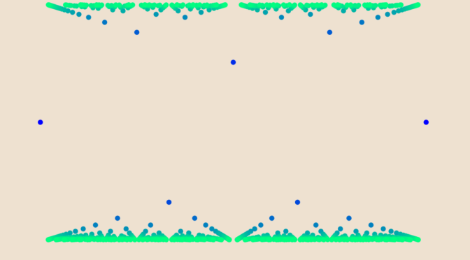
The function \(g\) defined on \([0,1]\) by \[
g(x)=\begin{cases}
0 & \text{ if } x \notin \mathbb Q \text{ or if } x = 0\\
\frac{(-1)^q (q-1)}{q} & \text{ if } x = \frac{p}{q} \neq 0 \text{, with } p, q \text{ relatively prime}
\end{cases}\] is bounded, as for \(x \in \mathbb Q \cap [0,1]\) we have \[
\left\vert g(x) \right\vert < 1.\] Hence \(g\) takes values in the interval \([-1,1]\). We prove that the infimum of \(g\) is \(-1\) and its supremum \(1\) on all intervals \([a,b]\) with \(0 < a < b <1\). Consider \(\varepsilon > 0\) and an odd prime \(q\) such that \[
q > \max(\frac{1}{\varepsilon}, \frac{1}{b-a}).\] This is possible as there are infinitely many prime numbers. By the pigeonhole principle and as \(0 < \frac{1}{q} < b-a\), there exists a natural number \(p\) such that \(\frac{p}{q} \in (a,b)\). We have \[ -1 < g \left(\frac{p}{q} \right) = \frac{(-1)^q (q-1)}{q} = - \frac{q-1}{q} <-1 +\varepsilon\] as \(q\) is supposed to be an odd prime with \(q > \frac{1}{\varepsilon}\). This proves that the infimum of \(g\) is \(-1\). By similar arguments, one can prove that the supremum of \(g\) on \([a,b]\) is \(1\).

On limit at infinity of functions and their derivatives

We consider continuously differentiable real functions defined on \((0,\infty)\) and the limits \[
\lim\limits_{x \to \infty} f(x) \text{ and } \lim\limits_{x \to \infty} f^\prime(x).\]

A map \(f\) such that \(\lim\limits_{x \to \infty} f(x) = \infty\) and \(\lim\limits_{x \to \infty} f^\prime(x) = 0\)

Consider the map \(f : x \mapsto \sqrt{x}\). It is clear that \(\lim\limits_{x \to \infty} f(x) = \infty\). As \(f^\prime(x) = \frac{1}{2 \sqrt{x}}\), we have as announced \(\lim\limits_{x \to \infty} f^\prime(x) = 0\)

A bounded map \(g\) having no limit at infinity such that \(\lim\limits_{x \to \infty} g^\prime(x) = 0\)

One idea is to take an oscillating map whose wavelength is increasing to \(\infty\). Let’s take the map \(g : x \mapsto \cos \sqrt{x}\). \(g\) doesn’t have a limit at \(\infty\) as for \(n \in \mathbb N\), we have \(g(n^2 \pi^2) = \cos n \pi = (-1)^n\). However, the derivative of \(g\) is \[
g^\prime(x) = – \frac{\sin \sqrt{x}}{2 \sqrt{x}},\] and as \(\vert g^\prime(x) \vert \le \frac{1}{2 \sqrt{x}}\) for all \(x \in (0,\infty)\), we have \(\lim\limits_{x \to \infty} g^\prime(x) = 0\).

Limit points of real sequences

Let’s start by recalling an important theorem of real analysis:

THEOREM. A necessary and sufficient condition for the convergence of a real sequence is that it is bounded and has a unique limit point.

As a consequence of the theorem, a sequence having a unique limit point is divergent if it is unbounded. An example of such a sequence is the sequence \[
u_n = \frac{n}{2}(1+(-1)^n),\] whose initial values are \[
0, 1, 0, 2, 0, 3, 0, 4, 0, 5, 6, \dots\] \((u_n)\) is an unbounded sequence whose unique limit point is \(0\).

Let’s now look at sequences having more complicated limit points sets.

A sequence whose set of limit points is the set of natural numbers

Consider the sequence \((v_n)\) whose initial terms are \[
1, 1, 2, 1, 2, 3, 1, 2, 3, 4, 1, 2, 3, 4, 5, \dots\] \((v_n)\) is defined as follows \[
v_n=\begin{cases}
1 &\text{ for } n= 1\\
n – \frac{k(k+1)}{2} &\text{ for } \frac{k(k+1)}{2} \lt n \le \frac{(k+1)(k+2)}{2}
\end{cases}\] \((v_n)\) is well defined as the sequence \((\frac{k(k+1)}{2})_{k \in \mathbb N}\) is strictly increasing with first term equal to \(1\). \((v_n)\) is a sequence of natural numbers. As \(\mathbb N\) is a set of isolated points of \(\mathbb R\), we have \(V \subseteq \mathbb N\), where \(V\) is the set of limit points of \((v_n)\). Conversely, let’s take \(m \in \mathbb N\). For \(k + 1 \ge m\), we have \(\frac{k(k+1)}{2} + m \le \frac{(k+1)(k+2)}{2}\), hence \[
u_{\frac{k(k+1)}{2} + m} = m\] which proves that \(m\) is a limit point of \((v_n)\). Finally the set of limit points of \((v_n)\) is the set of natural numbers.

Continue reading Limit points of real sequences

A linear map without any minimal polynomial

Given an endomorphism \(T\) on a finite-dimensional vector space \(V\) over a field \(\mathbb F\), the minimal polynomial \(\mu_T\) of \(T\) is well defined as the generator (unique up to units in \(\mathbb F\)) of the ideal:\[
I_T= \{p \in \mathbb F[t]\ ; \ p(T)=0\}.\]

For infinite-dimensional vector spaces, the minimal polynomial might not be defined. Let’s provide an example.

We take the real polynomials \(V = \mathbb R [t]\) as a real vector space and consider the derivative map \(D : P \mapsto P^\prime\). Let’s prove that \(D\) doesn’t have any minimal polynomial. By contradiction, suppose that \[
\mu_D(t) = a_0 + a_1 t + \dots + a_n t^n \text{ with } a_n \neq 0\] is the minimal polynomial of \(D\), which means that for all \(P \in \mathbb R[t]\) we have \[
a_0 + a_1 P^\prime + \dots + a_n P^{(n)} = 0.\] Taking for \(P\) the polynomial \(t^n\) we get \[
a_0 t^n + n a_1 t^{n-1} + \dots + n! a_n = 0,\] which doesn’t make sense as \(n! a_n \neq 0\), hence \(a_0 t^n + n a_1 t^{n-1} + \dots + n! a_n\) cannot be the zero polynomial.

We conclude that \(D\) doesn’t have any minimal polynomial.

Non linear map preserving Euclidean norm

Let \(V\) be a real vector space endowed with an Euclidean norm \(\Vert \cdot \Vert\).

A bijective map \( T : V \to V\) that preserves inner product \(\langle \cdot, \cdot \rangle\) is linear. Also, Mazur-Ulam theorem states that an onto map \( T : V \to V\) which is an isometry (\( \Vert T(x)-T(y) \Vert = \Vert x-y \Vert \) for all \(x,y \in V\)) and fixes the origin (\(T(0) = 0\)) is linear.

What about an application that preserves the norm (\(\Vert T(x) \Vert = \Vert x \Vert\) for all \(x \in V\))? \(T\) might not be linear as we show with following example:\[
\begin{array}{l|rcll}
T : & V & \longrightarrow & V \\
& x & \longmapsto & x & \text{if } \Vert x \Vert \neq 1\\
& x & \longmapsto & -x & \text{if } \Vert x \Vert = 1\end{array}\]

It is clear that \(T\) preserves the norm. However \(T\) is not linear as soon as \(V\) is not the zero vector space. In that case, consider \(x_0\) such that \(\Vert x_0 \Vert = 1\). We have:\[
\begin{cases}
T(2 x_0) &= 2 x_0 \text{ as } \Vert 2 x_0 \Vert = 2\\
\text{while}\\
T(x_0) + T(x_0) = -x_0 + (-x_0) &= – 2 x_0
\end{cases}\]

Non linear map preserving orthogonality

Let \(V\) be a real vector space endowed with an inner product \(\langle \cdot, \cdot \rangle\).

It is known that a bijective map \( T : V \to V\) that preserves the inner product \(\langle \cdot, \cdot \rangle\) is linear.

That might not be the case if \(T\) is supposed to only preserve orthogonality. Let’s consider for \(V\) the real plane \(\mathbb R^2\) and the map \[
\begin{array}{l|rcll}
T : & \mathbb R^2 & \longrightarrow & \mathbb R^2 \\
& (x,y) & \longmapsto & (x,y) & \text{for } xy \neq 0\\
& (x,0) & \longmapsto & (0,x)\\
& (0,y) & \longmapsto & (y,0) \end{array}\]

The restriction of \(T\) to the plane less the x-axis and the y-axis is the identity and therefore is bijective on this set. Moreover \(T\) is a bijection from the x-axis onto the y-axis, and a bijection from the y-axis onto the x-axis. This proves that \(T\) is bijective on the real plane.

\(T\) preserves the orthogonality on the plane less x-axis and y-axis as it is the identity there. As \(T\) swaps the x-axis and the y-axis, it also preserves orthogonality of the coordinate axes. However, \(T\) is not linear as for non zero \(x \neq y\) we have: \[
\begin{cases}
T[(x,0) + (0,y)] = T[(x,y)] &= (x,y)\\
\text{while}\\
T[(x,0)] + T[(0,y)] = (0,x) + (y,0) &= (y,x)
\end{cases}\]

The line with two origins

Let’s introduce and describe some properties of the line with two origins.

Let \(X\) be the union of the set \(\mathbb R \setminus \{0\}\) and the two-point set \(\{p,q\}\). The line with two origins is the set \(X\) topologized by taking as base the collection \(\mathcal B\) of all open intervals in \(\mathbb R\) that do not contain \(0\), along with all sets of the form \((-a,0) \cup \{p\} \cup (0,a)\) and all sets of the form \((-a,0) \cup \{q\} \cup (0,a)\), for \(a > 0\).

\(\mathcal B\) is a base for a topology \(\mathcal T\) of \(X\)

Indeed, one can verify that the elements of \(\mathcal B\) cover \(X\) as \[
X = \left( \bigcup_{a > 0} (-a,0) \cup \{p\} \cup (0,a) \right) \cup \left( \bigcup_{a > 0} (-a,0) \cup \{q\} \cup (0,a) \right)\] and that the intersection of two elements of \(\mathcal B\) is the union of elements of \(\mathcal B\) (verification left to the reader).

Each of the spaces \(X \setminus \{p\}\) and \(X \setminus \{q\}\) is homeomorphic to \(\mathbb R\)

Let’s prove it for \(X \setminus \{p\}\). The map \[
\begin{array}{l|rcll}
f : & X \setminus \{p\} & \longrightarrow & \mathbb R \\
& x & \longmapsto & x & \text{for } x \neq q\\
& q & \longmapsto & 0 \end{array}\] is a bijection. \(f\) is continuous as the inverse image of an open interval \(I\) of \(\mathbb R\) is an open subset of \(X\). For example taking \(I=(-b,c)\) with \(0 < b < c\), we have \begin{align*} f^{-1}[I] &= (-b,0) \cup \{q\} \cup (0,c)\\ &= \left( (-b,0) \cup \{q\} \cup (0,b) \right) \cup (b/2,c) \end{align*} One can also prove that \(f^{-1}\) is continuous. Continue reading The line with two origins

A power series converging everywhere on its circle of convergence defining a non-continuous function

Consider a complex power series \(\displaystyle \sum_{k=0}^\infty a_k z^k\) with radius of convergence \(0 \lt R \lt \infty\) and suppose that for every \(w\) with \(\vert w \vert = R\), \(\displaystyle \sum_{k=0}^\infty a_k w^k\) converges.

We provide an example where the power expansion at the origin \[
\displaystyle f(z) = \sum_{k=0}^\infty a_k z^k\] is discontinuous on the closed disk \(\vert z \vert \le R \).

The function \(f\) is constructed as an infinite sum \[
\displaystyle f(z) = \sum_{n=1}^\infty f_n(z)\] with \(f_n(z) = \frac{\delta_n}{a_n-z}\) where \((\delta_n)_{n \in \mathbb N}\) is a sequence of positive real numbers and \((a_n)\) a sequence of complex numbers of modulus larger than one and converging to one. Let \(f_n^{(r)}(z)\) denote the sum of the first \(r\) terms in the power series expansion of \(f_n(z)\) and \(\displaystyle f^{(r)}(z) \equiv \sum_{n=1}^\infty f_n^{(r)}(z)\).

We’ll prove that:

  1. If \(\sum_n \delta_n \lt \infty\) then \(\sum_{n=1}^\infty f_n^{(r)}(z)\) converges and \(f(z) = \lim\limits_{r \to \infty} \sum_{n=1}^\infty f_n^{(r)}(z)\) for \(\vert z \vert \le 1\) and \(z \neq 1\).
  2. If \(a_n=1+i \epsilon_n\) and \(\sum_n \delta_n/\epsilon_n < \infty\) then \(\sum_{n=1}^\infty f_n^{(r)}(1)\) converges and \(f(1) = \lim\limits_{r \to \infty} \sum_{n=1}^\infty f_n^{(r)}(1)\)
  3. If \(\delta_n/\epsilon_n^2 \to \infty\) then \(f(z)\) is unbounded on the disk \(\vert z \vert \le 1\).

First, let’s recall this corollary of Lebesgue’s dominated convergence theorem:

Let \((u_{n,i})_{(n,i) \in \mathbb N \times \mathbb N}\) be a double sequence of complex numbers. Suppose that \(u_{n,i} \to v_i\) for all \(i\) as \(n \to \infty\), and that \(\vert u_{n,i} \vert \le w_i\) for all \(n\) with \(\sum_i w_i < \infty\). Then for all \(n\) the series \(\sum_i u_{n,i}\) is absolutely convergent and \(\lim_n \sum_i u_{n,i} = \sum_i v_i\).
Continue reading A power series converging everywhere on its circle of convergence defining a non-continuous function

A linear map having all numbers as eigenvalue

Consider a linear map \(\varphi : E \to E\) where \(E\) is a linear space over the field \(\mathbb C\) of the complex numbers. When \(E\) is a finite dimensional vector space of dimension \(n \ge 1\), the number of eigenvalues is finite. The eigenvalues are the roots of the characteristic polynomial \(\chi_\varphi\) of \(\varphi\). \(\chi_\varphi\) is a complex polynomial of degree \(n \ge 1\). Therefore the set of eigenvalues of \(\varphi\) is non-empty and its cardinal is less than \(n\).

Things are different when \(E\) is an infinite dimensional space.

A linear map having all numbers as eigenvalue

Let’s consider the linear space \(E=\mathcal C^\infty([0,1])\) of smooth complex functions having derivatives of all orders and defined on the segment \([0,1]\). \(E\) is an infinite dimensional space: it contains all the polynomial maps.

On \(E\), we define the linear map \[\begin{array}{l|rcl}
\varphi : & \mathcal C^\infty([0,1]) & \longrightarrow & \mathcal C^\infty([0,1]) \\
& f & \longmapsto & f^\prime \end{array}\]

The set of eigenvalues of \(\varphi\) is all \(\mathbb C\). Indeed, for \(\lambda \in \mathbb C\) the map \(t \mapsto e^{\lambda t}\) is an eigenvector associated to the eigenvalue \(\lambda\).

A linear map having no eigenvalue

On the same linear space \(E=\mathcal C^\infty([0,1])\), we now consider the linear map \[\begin{array}{l|rcl}
\psi : & \mathcal C^\infty([0,1]) & \longrightarrow & \mathcal C^\infty([0,1]) \\
& f & \longmapsto & x f \end{array}\]

Suppose that \(\lambda \in \mathbb C\) is an eigenvalue of \(\psi\) and \(h \in E\) an eigenvector associated to \(\lambda\). By hypothesis, there exists \(x_0 \in [0,1]\) such that \(h(x_0) \neq 0\). Even better, as \(h\) is continuous, \(h\) is non-vanishing on \(J \cap [0,1]\) where \(J\) is an open interval containing \(x_0\). On \(J \cap [0,1]\) we have the equality \[
(\psi(h))(x) = x h(x) = \lambda h(x)\] Hence \(x=\lambda\) for all \(x \in J \cap [0,1]\). A contradiction proving that \(\psi\) has no eigenvalue.

A strictly increasing map that is not one-to-one

Consider two partially ordered sets \((E,\le)\) and \((F,\le)\) and a strictly increasing map \(f : E \to F\). If the order \((E,\le)\) is total, then \(f\) is one-to-one. Indeed for distinct elements \(x,y \in E\), we have either \(x < y\) or \(y < x\) and consequently \(f(x) < f(y)\) or \(f(y) < f(x)\). Therefore \(f(x)\) and \(f(y)\) are different. This is not true anymore for a partial order \((E,\le)\). We give a counterexample.

Consider a finite set \(E\) having at least two elements and partially ordered by the inclusion. Let \(f\) be the map defined on the powerset \(\wp(E)\) that maps \(A \subseteq E\) to its cardinal \(\vert A \vert \). \(f\) is obviously strictly increasing. However \(f\) is not one-to-one as for distincts elements \(a,b \in E\) we have \[
f(\{a\}) = 1 = f(\{b\})\]