Around bounded sets, greatest element and supremum

Consider a linearly ordered set \((X, \le)\) and a subset \(S \subseteq X\). Let’s recall some definitions:

  • \(S\) is bounded above if there exists an element \(k \in X\) such that \(k \ge s\) for all \(s \in S\).
  • \(g\) is a greatest element of \(S\) is \(g \in S\) and \(g \ge s\) for all \(s \in S\). \(l\) is a lowest element of \(S\) is \(l \in S\) and \(l \le s\) for all \(s \in S\).
  • \(a\) is an supremum of \(S\) if it is the least element in \(X\) that is greater than or equal to all elements of \(S\).

Subsets with a supremum but no greatest element

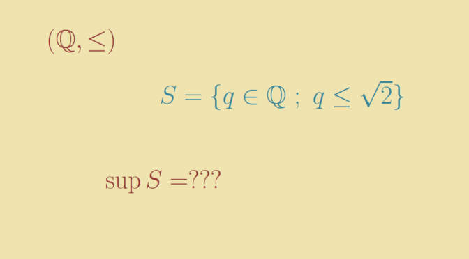
Let’s give examples of subsets having a supremum but no greatest element. First consider the ordered set \((\mathbb R, \le)\) and the subset \(S=\{ q \in \mathbb Q \ ; \ q \le \sqrt{2}\}\). \(S\) is bounded above by \(2\). \(\sqrt{2}\) is a supremum of \(S\) as we have \(q \le \sqrt{2}\) for all \(q \in S\) and as for \(b < \sqrt{2}\), it exists \(q \in \mathbb Q\) such that \(b < q < \sqrt{2}\) because \(\mathbb Q\) is dense in \(\mathbb R\). However \(S\) doesn't have a greatest element because \(\sqrt{2}\) is an irrational number.

For our second example we take \(X = \mathbb N \times \mathbb N\) ordered lexicographically by \(\preceq\). The subset \(S=\{(0,n) \ ; \ n \in \mathbb N\}\) is bounded above by \((2,0)\). Moreover \((1,0)\) is a supremum. But \(S\) doesn’t have a greatest element as for \((0,n) \in S\) we have \((0,n) \prec (0,n+1)\).

Bounded above subsets with no supremum

Leveraging the examples above, we take \((X, \le) = (\mathbb Q, \le)\) and \(S=\{ q \in \mathbb Q \ ; \ q \le \sqrt{2}\}\). \(S\) is bounded above, by \(2\) for example. However \(S\) doesn’t have a supremum because \(\sqrt{2} \notin \mathbb Q\).

Another example is the set \(X = \mathbb N \times \mathbb Z\) ordered lexicographically by \(\preceq\). The subset \(S=\{(0,n) \ ; \ n \in \mathbb N\}\) is bounded above by \((2,0)\) but has no supremum. Indeed, the elements greater or equal to all the elements of \(S\) are the elements \((a,b)\) with \(a \ge 1\). However \((a,b)\) with \(a \ge 1\) cannot be a supremum of \(S\), as \((a,b-1) \prec (a,b)\) and \((a,b-1)\) is greater than all the elements of \(S\).

Counterexample around infinite products

Let’s recall two theorems about infinite products \(\prod \ (1+a_n)\). The first one deals with nonnegative terms \(a_n\).

THEOREM 1 An infinite product \(\prod \ (1+a_n)\) with nonnegative terms \(a_n\) converges if and only if the series \(\sum a_n\) converges.

The second is related to infinite products with complex terms.

THEOREM 2 The absolute convergence of the series \(\sum a_n\) implies the convergence of the infinite product \(\prod \ (1+a_n)\). Moreover \(\prod \ (1+a_n)\) is not zero providing \(a_n \neq -1\) for all \(n \in \mathbb N\).

The converse of Theorem 2 is not true as shown by following counterexample.

We consider \(a_n=(-1)^n/(n+1)\). For \(N \in \mathbb N\) we have:
\[\prod_{n=1}^N \ (1+a_n) =
\begin{cases}
\frac{1}{2} &\text{ for } N \text{ odd}\\
\frac{1}{2}(1+\frac{1}{N+1}) &\text{ for } N \text{ even}
\end{cases}
\] hence the infinite product \(\prod \ (1+a_n)\) converges (to \(\frac{1}{2}\)) while the series \(\sum \left\vert a_n \right\vert = \sum \frac{1}{n+1}\) diverges (it is the harmonic series with first term omitted).

Counterexample around L’Hôpital’s rule

Let us consider two differentiable functions \(f\) and \(g\) defined in an open interval \((a,b)\), where \(b\) might be \(\infty\). If
\[\lim\limits_{x \to b^-} f(x) = \lim\limits_{x \to b^-} g(x) = \infty\] and if \(g^\prime(x) \neq 0\) in some interval \((c,b)\), then a version of l’Hôpital’s rule states that \(\lim\limits_{x \to b^-} \frac{f^\prime(x)}{g^\prime(x)} = L\) implies \(\lim\limits_{x \to b^-} \frac{f(x)}{g(x)} = L\).

We provide a counterexample when \(g^\prime\) vanishes in all neighborhood of \(b\). The counterexample is due to the Austrian mathematician Otto Stolz.

We take \((0,\infty)\) for the interval \((a,b)\) and \[
\begin{cases}
f(x) &= x + \cos x \sin x\\
g(x) &= e^{\sin x}(x + \cos x \sin x)
\end{cases}\] which derivatives are \[
\begin{cases}
f^\prime(x) &= 2 \cos^2 x\\
g^\prime(x) &= e^{\sin x} \cos x (x + \cos x \sin x + 2 \cos x)
\end{cases}\] We have \[
\lim\limits_{x \to \infty} \frac{f^\prime(x)}{g^\prime(x)} = \lim\limits_{x \to \infty} \frac{2 \cos x}{e^{\sin x} (x + \cos x \sin x + 2 \cos x)} = 0,\] however \[
\frac{f(x)}{g(x)} = \frac{1}{e^{\sin x}}\] doesn’t have any limit at \(\infty\) as it oscillates between \(\frac{1}{e}\) and \(e\).

The Schwarz lantern

Consider a smooth curve defined by a continuous map \(f : [0,1] \to \mathbb R^n\) with \(n \ge 2\) where \(f\) is supposed to have a continuous derivative. One can prove that the curve is rectifiable, its arc length being \[
L = \lim\limits_{n \to \infty} \sum_{i=1}^n \vert f(t_i) – f(t_{i-1}) \vert = \int_0^1 \vert f^\prime (t) \vert \ dt\] with \(t_i = \frac{i}{n}\) for \(0 \le i \le n\).

What can happen when we consider a surface instead of a curve?

Consider a compact, smooth surface (possibly with boundary) embedded in \(\mathbb R^3\). We can approximate it as a polyhedral surface composed of small triangles with all vertices on the initial surface. Will the sum of the areas of the triangles converges to the area of the surface if their size is converging to zero?

The answer is negative and we provide a counterexample named Schwarz lantern. We take a cylinder of radius \(r\) and height \(h\). We approximate the cylinder by \(4nm\) isosceles triangles positioned as in the picture in \(2n\) slices. All triangles have the same base and height given by \[
b = 2r \sin \left(\frac{\pi}{m}\right), \ h = \sqrt{r^2 \left[1-\cos \left(\frac{\pi}{m}\right)\right]^2+\left(\frac{h}{2n}\right)^2}\] Hence the area of the polyhedral surface is \[
\begin{aligned}
S^\prime(m,n) &= 4 m n r \sin \left(\frac{\pi}{m}\right) \sqrt{r^2 \left[1-\cos \left(\frac{\pi}{m}\right)\right]^2+\left(\frac{h}{2n}\right)^2}\\
&= 4 m n r \sin \left(\frac{\pi}{m}\right) \sqrt{4 r^2 \sin^4 \left(\frac{\pi}{2m} \right)+\left(\frac{h}{2n}\right)^2}
\end{aligned}\] From there, let’s have a look to the value of \(S^\prime(m,n)\) as \(m,n \to \infty\).

Continue reading The Schwarz lantern

Counterexamples around Lebesgue’s Dominated Convergence Theorem

Let’s recall Lebesgue’s Dominated Convergence Theorem. Let \((f_n)\) be a sequence of real-valued measurable functions on a measure space \((X, \Sigma, \mu)\). Suppose that the sequence converges pointwise to a function \(f\) and is dominated by some integrable function \(g\) in the sense that \[
\vert f_n(x) \vert \le g (x)\] for all \(n \in \mathbb N\) and all \(x \in X\).
Then \(f\) is integrable and \[
\lim\limits_{n \to \infty} \int_X f_n(x) \ d \mu = \int_X f(x) \ d \mu\]

Let’s see what can happen if we drop the domination condition.

We consider the space \(\mathbb R\) endowed with Lebesgue measure and for \(E \subseteq \mathbb R\) we denote by \(\chi_E\) the indicator function of \(E\) defined by \[
\chi_E(x)=\begin{cases}
1 \text{ if } x \in E\\
0 \text{ otherwise}\end{cases}\] For \(n \in \mathbb N\), the function \(f_n=\frac{1}{2n}\chi_{(n^2-n,n^2+n)}\) is measurable and we have \[
\int_{\mathbb R} \frac{1}{2n}\chi_{(n^2-n,n^2+n)}(x) \ dx = \int_{n^2-n}^{n^2+n} \frac{1}{2n} \ dx = 1\] The sequence \((f_n)\) converges uniformly (and therefore pointwise) to the always vanishing function as for \(n \in \mathbb N\) we have for all \(x \in \mathbb R\) \(\vert f_n(x) \vert \le \frac{1}{2n}\). Hence the conclusion of Lebesgue’s Dominated Convergence Theorem doesn’t hold for the sequence \((f_n)\).

Let’s verify that the sequence \((f_n)\) is not dominated by some integrable function \(g\). For \(p < q\) integers, we have \[ \begin{aligned} q^2-q-(p^2+p) &= q^2-p^2 -q-p\\ &= (q-p)(q+p) -q -p\\ &\ge (q+p) -q-p=0 \end{aligned}\] Hence for \(p \neq q\) integers the intervals \((p^2-p,p^2+p)\) and \((q^2-q,q^2+q)\) are disjoint. Consequently for all \(x \in \mathbb R\) the sum \(\sum_{n \in \mathbb N} f_n(x)\) amounts to only one term and the function \(\sum_{n \in \mathbb N} f_n\) is well defined. If \(g\) dominates the sequence \((f_n)\), it satisfies \(0 \le \sum_{n \in \mathbb N} f_n \le g\). But \[ \int_{\mathbb R} \sum_{n \in \mathbb N} f_n(x) \ dx = \sum_{n \in \mathbb N} \int_{\mathbb R} f_n(x) \ dx = \sum_{n \in \mathbb N} 1 = \infty\] and \(g\) cannot be integrable. Continue reading Counterexamples around Lebesgue’s Dominated Convergence Theorem

Bounded functions and infimum, supremum

According to the extreme value theorem, a continuous real-valued function \(f\) in the closed and bounded interval \([a,b]\) must attain a maximum and a minimum, each at least once.

Let’s see what can happen for non-continuous functions. We consider below maps defined on \([0,1]\).

First let’s look at \[
f(x)=\begin{cases}
x &\text{ if } x \in (0,1)\\
1/2 &\text{otherwise}
\end{cases}\] \(f\) is bounded on \([0,1]\), continuous on the interval \((0,1)\) but neither at \(0\) nor at \(1\). The infimum of \(f\) is \(0\), its supremum \(1\), and \(f\) doesn’t attain those values. However, for \(0 < a < b < 1\), \(f\) attains its supremum and infimum on \([a,b]\) as \(f\) is continuous on this interval.

Bounded function that doesn’t attain its infimum and supremum on all \([a,b] \subseteq [0,1]\)

The function \(g\) defined on \([0,1]\) by \[
g(x)=\begin{cases}
0 & \text{ if } x \notin \mathbb Q \text{ or if } x = 0\\
\frac{(-1)^q (q-1)}{q} & \text{ if } x = \frac{p}{q} \neq 0 \text{, with } p, q \text{ relatively prime}
\end{cases}\] is bounded, as for \(x \in \mathbb Q \cap [0,1]\) we have \[
\left\vert g(x) \right\vert < 1.\] Hence \(g\) takes values in the interval \([-1,1]\). We prove that the infimum of \(g\) is \(-1\) and its supremum \(1\) on all intervals \([a,b]\) with \(0 < a < b <1\). Consider \(\varepsilon > 0\) and an odd prime \(q\) such that \[
q > \max(\frac{1}{\varepsilon}, \frac{1}{b-a}).\] This is possible as there are infinitely many prime numbers. By the pigeonhole principle and as \(0 < \frac{1}{q} < b-a\), there exists a natural number \(p\) such that \(\frac{p}{q} \in (a,b)\). We have \[ -1 < g \left(\frac{p}{q} \right) = \frac{(-1)^q (q-1)}{q} = - \frac{q-1}{q} <-1 +\varepsilon\] as \(q\) is supposed to be an odd prime with \(q > \frac{1}{\varepsilon}\). This proves that the infimum of \(g\) is \(-1\). By similar arguments, one can prove that the supremum of \(g\) on \([a,b]\) is \(1\).

On limit at infinity of functions and their derivatives

We consider continuously differentiable real functions defined on \((0,\infty)\) and the limits \[
\lim\limits_{x \to \infty} f(x) \text{ and } \lim\limits_{x \to \infty} f^\prime(x).\]

A map \(f\) such that \(\lim\limits_{x \to \infty} f(x) = \infty\) and \(\lim\limits_{x \to \infty} f^\prime(x) = 0\)

Consider the map \(f : x \mapsto \sqrt{x}\). It is clear that \(\lim\limits_{x \to \infty} f(x) = \infty\). As \(f^\prime(x) = \frac{1}{2 \sqrt{x}}\), we have as announced \(\lim\limits_{x \to \infty} f^\prime(x) = 0\)

A bounded map \(g\) having no limit at infinity such that \(\lim\limits_{x \to \infty} g^\prime(x) = 0\)

One idea is to take an oscillating map whose wavelength is increasing to \(\infty\). Let’s take the map \(g : x \mapsto \cos \sqrt{x}\). \(g\) doesn’t have a limit at \(\infty\) as for \(n \in \mathbb N\), we have \(g(n^2 \pi^2) = \cos n \pi = (-1)^n\). However, the derivative of \(g\) is \[
g^\prime(x) = – \frac{\sin \sqrt{x}}{2 \sqrt{x}},\] and as \(\vert g^\prime(x) \vert \le \frac{1}{2 \sqrt{x}}\) for all \(x \in (0,\infty)\), we have \(\lim\limits_{x \to \infty} g^\prime(x) = 0\).

Limit points of real sequences

Let’s start by recalling an important theorem of real analysis:

THEOREM. A necessary and sufficient condition for the convergence of a real sequence is that it is bounded and has a unique limit point.

As a consequence of the theorem, a sequence having a unique limit point is divergent if it is unbounded. An example of such a sequence is the sequence \[
u_n = \frac{n}{2}(1+(-1)^n),\] whose initial values are \[
0, 1, 0, 2, 0, 3, 0, 4, 0, 5, 6, \dots\] \((u_n)\) is an unbounded sequence whose unique limit point is \(0\).

Let’s now look at sequences having more complicated limit points sets.

A sequence whose set of limit points is the set of natural numbers

Consider the sequence \((v_n)\) whose initial terms are \[
1, 1, 2, 1, 2, 3, 1, 2, 3, 4, 1, 2, 3, 4, 5, \dots\] \((v_n)\) is defined as follows \[
v_n=\begin{cases}
1 &\text{ for } n= 1\\
n – \frac{k(k+1)}{2} &\text{ for } \frac{k(k+1)}{2} \lt n \le \frac{(k+1)(k+2)}{2}
\end{cases}\] \((v_n)\) is well defined as the sequence \((\frac{k(k+1)}{2})_{k \in \mathbb N}\) is strictly increasing with first term equal to \(1\). \((v_n)\) is a sequence of natural numbers. As \(\mathbb N\) is a set of isolated points of \(\mathbb R\), we have \(V \subseteq \mathbb N\), where \(V\) is the set of limit points of \((v_n)\). Conversely, let’s take \(m \in \mathbb N\). For \(k + 1 \ge m\), we have \(\frac{k(k+1)}{2} + m \le \frac{(k+1)(k+2)}{2}\), hence \[
u_{\frac{k(k+1)}{2} + m} = m\] which proves that \(m\) is a limit point of \((v_n)\). Finally the set of limit points of \((v_n)\) is the set of natural numbers.

Continue reading Limit points of real sequences

A linear map without any minimal polynomial

Given an endomorphism \(T\) on a finite-dimensional vector space \(V\) over a field \(\mathbb F\), the minimal polynomial \(\mu_T\) of \(T\) is well defined as the generator (unique up to units in \(\mathbb F\)) of the ideal:\[
I_T= \{p \in \mathbb F[t]\ ; \ p(T)=0\}.\]

For infinite-dimensional vector spaces, the minimal polynomial might not be defined. Let’s provide an example.

We take the real polynomials \(V = \mathbb R [t]\) as a real vector space and consider the derivative map \(D : P \mapsto P^\prime\). Let’s prove that \(D\) doesn’t have any minimal polynomial. By contradiction, suppose that \[
\mu_D(t) = a_0 + a_1 t + \dots + a_n t^n \text{ with } a_n \neq 0\] is the minimal polynomial of \(D\), which means that for all \(P \in \mathbb R[t]\) we have \[
a_0 + a_1 P^\prime + \dots + a_n P^{(n)} = 0.\] Taking for \(P\) the polynomial \(t^n\) we get \[
a_0 t^n + n a_1 t^{n-1} + \dots + n! a_n = 0,\] which doesn’t make sense as \(n! a_n \neq 0\), hence \(a_0 t^n + n a_1 t^{n-1} + \dots + n! a_n\) cannot be the zero polynomial.

We conclude that \(D\) doesn’t have any minimal polynomial.

Non linear map preserving Euclidean norm

Let \(V\) be a real vector space endowed with an Euclidean norm \(\Vert \cdot \Vert\).

A bijective map \( T : V \to V\) that preserves inner product \(\langle \cdot, \cdot \rangle\) is linear. Also, Mazur-Ulam theorem states that an onto map \( T : V \to V\) which is an isometry (\( \Vert T(x)-T(y) \Vert = \Vert x-y \Vert \) for all \(x,y \in V\)) and fixes the origin (\(T(0) = 0\)) is linear.

What about an application that preserves the norm (\(\Vert T(x) \Vert = \Vert x \Vert\) for all \(x \in V\))? \(T\) might not be linear as we show with following example:\[
\begin{array}{l|rcll}
T : & V & \longrightarrow & V \\
& x & \longmapsto & x & \text{if } \Vert x \Vert \neq 1\\
& x & \longmapsto & -x & \text{if } \Vert x \Vert = 1\end{array}\]

It is clear that \(T\) preserves the norm. However \(T\) is not linear as soon as \(V\) is not the zero vector space. In that case, consider \(x_0\) such that \(\Vert x_0 \Vert = 1\). We have:\[
\begin{cases}
T(2 x_0) &= 2 x_0 \text{ as } \Vert 2 x_0 \Vert = 2\\
\text{while}\\
T(x_0) + T(x_0) = -x_0 + (-x_0) &= – 2 x_0
\end{cases}\]

Mathematical exceptions to the rules or intuition