Category Archives: Analysis

Uniform continuous function but not Lipschitz continuous

Consider the function \[
\begin{array}{l|rcl}
f : & [0,1] & \longrightarrow & [0,1] \\
& x & \longmapsto & \sqrt{x} \end{array}\]

\(f\) is continuous on the compact interval \([0,1]\). Hence \(f\) is uniform continuous on that interval according to Heine-Cantor theorem. For a direct proof, one can verify that for \(\epsilon > 0\), one have \(\vert \sqrt{x} – \sqrt{y} \vert \le \epsilon\) for \(\vert x – y \vert \le \epsilon^2\).

However \(f\) is not Lipschitz continuous. If \(f\) was Lipschitz continuous for a Lipschitz constant \(K > 0\), we would have \(\vert \sqrt{x} – \sqrt{y} \vert \le K \vert x – y \vert\) for all \(x,y \in [0,1]\). But we get a contradiction taking \(x=0\) and \(y=\frac{1}{4 K^2}\) as \[
\vert \sqrt{x} – \sqrt{y} \vert = \frac{1}{2 K} > \frac{1}{4 K} = K \vert x – y \vert\]

Raabe-Duhamel’s test

The Raabe-Duhamel’s test (also named Raabe’s test) is a test for the convergence of a series \[
\sum_{n=1}^\infty a_n \] where each term is a real or complex number. The Raabe-Duhamel’s test was developed by Swiss mathematician Joseph Ludwig Raabe.

It states that if:

\[\displaystyle \lim _{n\to \infty }\left\vert{\frac {a_{n}}{a_{n+1}}}\right\vert=1 \text{ and } \lim _{{n\to \infty }} n \left(\left\vert{\frac {a_{n}}{a_{{n+1}}}}\right\vert-1 \right)=R,\]
then the series will be absolutely convergent if \(R > 1\) and divergent if \(R < 1\). First one can notice that Raabe-Duhamel's test maybe conclusive in cases where ratio test isn't. For instance, consider a real \(\alpha\) and the series \(u_n=\frac{1}{n^\alpha}\). We have \[ \lim _{n\to \infty } \frac{u_{n+1}}{u_n} = \lim _{n\to \infty } \left(\frac{n}{n+1} \right)^\alpha = 1\] and therefore the ratio test is inconclusive. However \[ \frac{u_n}{u_{n+1}} = \left(\frac{n+1}{n} \right)^\alpha = 1 + \frac{\alpha}{n} + o \left(\frac{1}{n}\right)\] for \(n\) around \(\infty\) and \[ \lim _{{n\to \infty }} n \left(\frac {u_{n}}{u_{{n+1}}}-1 \right)=\alpha.\] Raabe-Duhamel's test allows to conclude that the series \(\sum u_n\) diverges for \(\alpha <1\) and converges for \(\alpha > 1\) as well known.

When \(R=1\) in the Raabe’s test, the series can be convergent or divergent. For example, the series above \(u_n=\frac{1}{n^\alpha}\) with \(\alpha=1\) is the harmonic series which is divergent.

On the other hand, the series \(v_n=\frac{1}{n \log^2 n}\) is convergent as can be proved using the integral test. Namely \[
0 \le \frac{1}{n \log^2 n} \le \int_{n-1}^n \frac{dt}{t \log^2 t} \text{ for } n \ge 3\] and \[
\int_2^\infty \frac{dt}{t \log^2 t} = \left[-\frac{1}{\log t} \right]_2^\infty = \frac{1}{\log 2}\] is convergent, while \[
\frac{v_n}{v_{n+1}} = 1 + \frac{1}{n} +\frac{2}{n \log n} + o \left(\frac{1}{n \log n}\right)\] for \(n\) around \(\infty\) and therefore \(R=1\) in the Raabe-Duhamel’s test.

Counterexamples around Cauchy condensation test

According to Cauchy condensation test: for a non-negative, non-increasing sequence \((u_n)_{n \in \mathbb N}\) of real numbers, the series \(\sum_{n \in \mathbb N} u_n\) converges if and only if the condensed series \(\sum_{n \in \mathbb N} 2^n u_{2^n}\) converges.

The test doesn’t hold for any non-negative sequence. Let’s have a look at counterexamples.

A sequence such that \(\sum_{n \in \mathbb N} u_n\) converges and \(\sum_{n \in \mathbb N} 2^n u_{2^n}\) diverges

Consider the sequence \[
u_n=\begin{cases}
\frac{1}{n} & \text{ for } n \in \{2^k \ ; \ k \in \mathbb N\}\\
0 & \text{ else} \end{cases}\] For \(n \in \mathbb N\) we have \[
0 \le \sum_{k = 1}^n u_k \le \sum_{k = 1}^{2^n} u_k = \sum_{k = 1}^{n} \frac{1}{2^k} < 1,\] therefore \(\sum_{n \in \mathbb N} u_n\) converges as its partial sums are positive and bounded above. However \[\sum_{k=1}^n 2^k u_{2^k} = \sum_{k=1}^n 1 = n,\] so \(\sum_{n \in \mathbb N} 2^n u_{2^n}\) diverges.

A sequence such that \(\sum_{n \in \mathbb N} v_n\) diverges and \(\sum_{n \in \mathbb N} 2^n v_{2^n}\) converges

Consider the sequence \[
v_n=\begin{cases}
0 & \text{ for } n \in \{2^k \ ; \ k \in \mathbb N\}\\
\frac{1}{n} & \text{ else} \end{cases}\] We have \[
\sum_{k = 1}^{2^n} v_k = \sum_{k = 1}^{2^n} \frac{1}{k} – \sum_{k = 1}^{n} \frac{1}{2^k} > \sum_{k = 1}^{2^n} \frac{1}{k} -1\] which proves that the series \(\sum_{n \in \mathbb N} v_n\) diverges as the harmonic series is divergent. However for \(n \in \mathbb N\), \(2^n v_{2^n} = 0 \) and \(\sum_{n \in \mathbb N} 2^n v_{2^n}\) converges.

Counterexamples around the Cauchy product of real series

Let \(\sum_{n = 0}^\infty a_n, \sum_{n = 0}^\infty b_n\) be two series of real numbers. The Cauchy product \(\sum_{n = 0}^\infty c_n\) is the series defined by \[
c_n = \sum_{k=0}^n a_k b_{n-k}\] According to the theorem of Mertens, if \(\sum_{n = 0}^\infty a_n\) converges to \(A\), \(\sum_{n = 0}^\infty b_n\) converges to \(B\) and at least one of the two series is absolutely convergent, their Cauchy product converges to \(AB\). This can be summarized by the equality \[
\left( \sum_{n = 0}^\infty a_n \right) \left( \sum_{n = 0}^\infty b_n \right) = \sum_{n = 0}^\infty c_n\]

The assumption stating that at least one of the two series converges absolutely cannot be dropped as shown by the example \[
\sum_{n = 0}^\infty a_n = \sum_{n = 0}^\infty b_n = \sum_{n = 0}^\infty \frac{(-1)^n}{\sqrt{n+1}}\] Those series converge according to Leibniz test, as the sequence \((1/\sqrt{n+1})\) decreases monotonically to zero. However, the Cauchy product is defined by \[
c_n=\sum_{k=0}^n \frac{(-1)^k}{\sqrt{k+1}} \cdot \frac{(-1)^{n-k}}{\sqrt{n-k+1}} = (-1)^n \sum_{k=0}^n \frac{1}{\sqrt{(k+1)(n-k+1)}}\] As we have \(1 \le k+ 1 \le n+1\) and \(1 \le n-k+ 1 \le n+1\) for \(k = 0 \dots n\), we get \(\frac{1}{\sqrt{(k+1)(n-k+1)}} \ge \frac{1}{n+1}\) and therefore \(\vert c_n \vert \ge 1\) proving that the Cauchy product of \(\sum_{n = 0}^\infty a_n\) and \(\sum_{n = 0}^\infty b_n\) diverges.

The Cauchy product may also converge while the initial series both diverge. Let’s consider \[
\begin{cases}
(a_n) = (2, 2, 2^2, \dots, 2^n, \dots)\\
(b_n) = (-1, 1, 1, 1, \dots)
\end{cases}\] The series \(\sum_{n = 0}^\infty a_n, \sum_{n = 0}^\infty b_n\) diverge. Their Cauchy product is the series defined by \[
c_n=\begin{cases}
-2 & \text{ for } n=0\\
0 & \text{ for } n>0
\end{cases}\] which is convergent.

A linear differential equation with no solution to an initial value problem


Consider a first order linear differential equation \[
y^\prime(x) = A(x)y(x) + B(x)\] where \(A, B\) are real continuous functions defined on a non-empty real interval \(I\). According to Picard-Lindelöf theorem, the initial value problem \[
\begin{cases}
y^\prime(x) = A(x)y(x) + B(x)\\
y(x_0) = y_0, \ x_0 \in I
\end{cases}\] has a unique solution defined on \(I\).

However, a linear differential equation \[
c(x)y^\prime(x) = A(x)y(x) + B(x)\] where \(A, B, c\) are real continuous functions might not have a solution to an initial value problem. Let’s have a look at the equation \[
x y^\prime(x) = y(x) \tag{E}\label{eq:IVP}\] for \(x \in \mathbb R\). The equation is linear.

For \(x \in (-\infty,0)\) a solution to \eqref{eq:IVP} is a solution of the explicit differential linear equation \[
y^\prime(x) = \frac{y(x)}x\] hence can be written \(y(x) = \lambda_-x\) with \(\lambda_- \in \mathbb R\). Similarly, a solution to \eqref{eq:IVP} on the interval \((0,\infty)\) is of the form \(y(x) = \lambda_+ x\) with \(\lambda_+ \in \mathbb R\).

A global solution to \eqref{eq:IVP}, i.e. defined on the whole real line is differentiable at \(0\) hence the equation \[
\lambda_- = y_-^\prime(0)=y_+^\prime(0) = \lambda_+\] which means that \(y(x) = \lambda x\) where \(\lambda=\lambda_-=\lambda_+\).

In particular all solutions defined on \(\mathbb R\) are such that \(y(0)=0\). Therefore the initial value problem \[
\begin{cases}
x y^\prime(x) = y(x)\\
y(0)=1
\end{cases}\] has no solution.

Pointwise convergence not uniform on any interval

We provide in this article an example of a pointwise convergent sequence of real functions that doesn’t converge uniformly on any interval.

Let’s consider a sequence \((a_p)_{p \in \mathbb N}\) enumerating the set \(\mathbb Q\) of rational numbers. Such a sequence exists as \(\mathbb Q\) is countable.

Now let \((g_n)_{n \in \mathbb N}\) be the sequence of real functions defined on \(\mathbb R\) by \[
g_n(x) = \sum_{p=1}^{\infty} \frac{1}{2^p} f_n(x-a_p)\] where \(f_n : x \mapsto \frac{n^2 x^2}{1+n^4 x^4}\) for \(n \in \mathbb N\).

\(f_n\) main properties

\(f_n\) is a rational function whose denominator doesn’t vanish. Hence \(f_n\) is indefinitely differentiable. As \(f_n\) is an even function, we can study it only on \([0,\infty)\).

We have \[
f_n^\prime(x)= 2n^2x \frac{1-n^4x^4}{(1+n^4 x^4)^2}.\] \(f_n^\prime\) vanishes at zero (like \(f_n\)) is positive on \((0,\frac{1}{n})\), vanishes at \(\frac{1}{n}\) and is negative on \((\frac{1}{n},\infty)\). Hence \(f_n\) has a maximum at \(\frac{1}{n}\) with \(f_n(\frac{1}{n}) = \frac{1}{2}\) and \(0 \le f_n(x) \le \frac{1}{2}\) for all \(x \in \mathbb R\).

Also for \(x \neq 0\) \[
0 \le f_n(x) =\frac{n^2 x^2}{1+n^4 x^4} \le \frac{n^2 x^2}{n^4 x^4} = \frac{1}{n^2 x^2}\] consequently \[
0 \le f_n(x) \le \frac{1}{n} \text{ for } x \ge \frac{1}{\sqrt{n}}.\]

\((g_n)\) converges pointwise to zero

First, one can notice that \(g_n\) is well defined. For \(x \in \mathbb R\) and \(p \in \mathbb N\) we have \(0 \le \frac{1}{2^p} f_n(x-a_p) \le \frac{1}{2^p} \cdot\ \frac{1}{2}=\frac{1}{2^{p+1}}\) according to previous paragraph. Therefore the series of functions \(\sum \frac{1}{2^p} f_n(x-a_p)\) is normally convergent. \(g_n\) is also continuous as for all \(p \in \mathbb N\) \(x \mapsto \frac{1}{2^p} f_n(x-a_p)\) is continuous. Continue reading Pointwise convergence not uniform on any interval

A differentiable real function with unbounded derivative around zero

Consider the real function defined on \(\mathbb R\)\[
f(x)=\begin{cases}
0 &\text{for } x = 0\\
x^2 \sin \frac{1}{x^2} &\text{for } x \neq 0
\end{cases}\]

\(f\) is continuous and differentiable on \(\mathbb R\setminus \{0\}\). For \(x \in \mathbb R\) we have \(\vert f(x) \vert \le x^2\), which implies that \(f\) is continuous at \(0\). Also \[
\left\vert \frac{f(x)-f(0)}{x} \right\vert = \left\vert x \sin \frac{1}{x^2} \right\vert \le \vert x \vert\] proving that \(f\) is differentiable at zero with \(f^\prime(0) = 0\). The derivative of \(f\) for \(x \neq 0\) is \[
f^\prime(x) = \underbrace{2x \sin \frac{1}{x^2}}_{=g(x)}-\underbrace{\frac{2}{x} \cos \frac{1}{x^2}}_{=h(x)}\] On the interval \((-1,1)\), \(g(x)\) is bounded by \(2\). However, for \(a_k=\frac{1}{\sqrt{k \pi}}\) with \(k \in \mathbb N\) we have \(h(a_k)=2 \sqrt{k \pi} (-1)^k\) which is unbounded while \(\lim\limits_{k \to \infty} a_k = 0\). Therefore \(f^\prime\) is unbounded in all neighborhood of the origin.

A Riemann-integrable map that is not regulated

For a Banach space \(X\), a function \(f : [a,b] \to X\) is said to be regulated if there exists a sequence of step functions \(\varphi_n : [a,b] \to X\) converging uniformly to \(f\).

One can prove that a regulated function \(f : [a,b] \to X\) is Riemann-integrable. Is the converse true? The answer is negative and we provide below an example of a Riemann-integrable real function that is not regulated. Let’s first prove following theorem.

THEOREM A bounded function \(f : [a,b] \to \mathbb R\) that is (Riemann) integrable on all intervals \([c, b]\) with \(a < c < b\) is integrable on \([a,b]\).

PROOF Take \(M > 0\) such that for all \(x \in [a,b]\) we have \(\vert f(x) \vert < M\). For \(\epsilon > 0\), denote \(c = \inf(a + \frac{\epsilon}{4M},b + \frac{b-a}{2})\). As \(f\) is supposed to be integrable on \([c,b]\), one can find a partition \(P\): \(c=x_1 < x_2 < \dots < x_n =b\) such that \(0 \le U(f,P) - L(f,P) < \frac{\epsilon}{2}\) where \(L(f,P),U(f,P)\) are the lower and upper Darboux sums. For the partition \(P^\prime\): \(a= x_0 < c=x_1 < x_2 < \dots < x_n =b\), we have \[ \begin{aligned} 0 \le U(f,P^\prime) - L(f,P^\prime) &\le 2M(c-a) + \left(U(f,P) - L(f,P)\right)\\ &< 2M \frac{\epsilon}{4M} + \frac{\epsilon}{2} = \epsilon \end{aligned}\] 
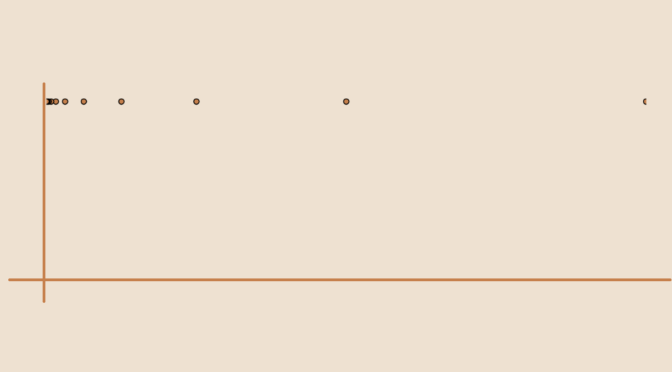
We now prove that the function \(f : [0,1] \to [0,1]\) defined by \[ f(x)=\begin{cases} 1 &\text{ if } x \in \{2^{-k} \ ; \ k \in \mathbb N\}\\ 0 &\text{otherwise} \end{cases}\] is Riemann-integrable (that follows from above theorem) and not regulated. Let's prove it. If \(f\) was regulated, there would exist a step function \(g\) such that \(\vert f(x)-g(x) \vert < \frac{1}{3}\) for all \(x \in [0,1]\). If \(0=x_0 < x_1 < \dots < x_n=1\) is a partition associated to \(g\) and \(c_1\) the value of \(g\) on the interval \((0,x_1)\), we must have \(\vert 1-c_1 \vert < \frac{1}{3}\) as \(f\) takes (an infinite number of times) the value \(1\) on \((0,x_1)\). But \(f\) also takes (an infinite number of times) the value \(0\) on \((0,x_1)\). Hence we must have \(\vert c_1 \vert < \frac{1}{3}\). We get a contradiction as those two inequalities are not compatible.

A discontinuous midpoint convex function

Let’s recall that a real function \(f: \mathbb R \to \mathbb R\) is called convex if for all \(x, y \in \mathbb R\) and \(\lambda \in [0,1]\) we have \[
f((1- \lambda) x + \lambda y) \le (1- \lambda) f(x) + \lambda f(y)\] \(f\) is called midpoint convex if for all \(x, y \in \mathbb R\) \[
f \left(\frac{x+y}{2}\right) \le \frac{f(x)+f(y)}{2}\] One can prove that a continuous midpoint convex function is convex. Sierpinski proved the stronger theorem, that a real-valued Lebesgue measurable function that is midpoint convex will be convex.

Can one find a discontinuous midpoint convex function? The answer is positive but requires the Axiom of Choice. Why? Because Robert M. Solovay constructed a model of Zermelo-Fraenkel set theory (ZF), exclusive of the axiom of choice where all functions are Lebesgue measurable. Hence convex according to Sierpinski theorem. And one knows that convex functions defined on \(\mathbb R\) are continuous.

Referring to my previous article on the existence of discontinuous additive map, let’s use a Hamel basis \(\mathcal B = (b_i)_{i \in I}\) of \(\mathbb R\) considered as a vector space on \(\mathbb Q\). Take \(i_1 \in I\), define \(f(i_1)=1\) and \(f(i)=0\) for \(i \in I\setminus \{i_1\}\) and extend \(f\) linearly on \(\mathbb R\). \(f\) is midpoint convex as it is linear. As the image of \(\mathbb R\) under \(f\) is \(\mathbb Q\), \(f\) is discontinuous as explained in the discontinuous additive map counterexample.

Moreover, \(f\) is unbounded on all open real subsets. By linearity, it is sufficient to prove that \(f\) is unbounded around \(0\). Let’s consider \(i_1 \neq i_2 \in I\). \(G= b_{i_1} \mathbb Z + b_{i_2} \mathbb Z\) is a proper subgroup of the additive \(\mathbb R\) group. Hence \(G\) is either dense of discrete. It cannot be discrete as the set of vectors \(\{b_1,b_2\}\) is linearly independent. Hence \(G\) is dense in \(\mathbb R\). Therefore, one can find a non vanishing sequence \((x_n)_{n \in \mathbb N}=(q_n^1 b_{i_1} + q_n^2 b_{i_2})_{n \in \mathbb N}\) (with \((q_n^1,q_n^2) \in \mathbb Q^2\) for all \(n \in \mathbb N\)) converging to \(0\). As \(\{b_1,b_2\}\) is linearly independent, this implies \(\vert q_n^1 \vert, \vert q_n^2 \vert \underset{n\to+\infty}{\longrightarrow} \infty\) and therefore \[
\lim\limits_{n \to \infty} \vert f(x_n) \vert = \lim\limits_{n \to \infty} \vert f(q_n^1 b_{i_1} + q_n^2 b_{i_2}) \vert = \lim\limits_{n \to \infty} \vert q_n^1 \vert = \infty.\]

A discontinuous additive map

A function \(f\) defined on \(\mathbb R\) into \(\mathbb R\) is said to be additive if and only if for all \(x, y \in \mathbb R\)
\[f(x+y) = f(x) + f(y).\] If \(f\) is supposed to be continuous at zero, \(f\) must have the form \(f(x)=cx\) where \(c=f(1)\). This can be shown using following steps:

  • \(f(0) = 0\) as \(f(0) = f(0+0)= f(0)+f(0)\).
  • For \(q \in \mathbb N\) \(f(1)=f(q \cdot \frac{1}{q})=q f(\frac{1}{q})\). Hence \(f(\frac{1}{q}) = \frac{f(1)}{q}\). Then for \(p,q \in \mathbb N\), \(f(\frac{p}{q}) = p f(\frac{1}{q})= f(1) \frac{p}{q}\).
  • As \(f(-x) = -f(x)\) for all \(x \in\mathbb R\), we get that for all rational number \(\frac{p}{q} \in \mathbb Q\), \(f(\frac{p}{q})=f(1)\frac{p}{q}\).
  • The equality \(f(x+y) = f(x) + f(y)\) implies that \(f\) is continuous on \(\mathbb R\) if it is continuous at \(0\).
  • We can finally conclude to \(f(x)=cx\) for all real \(x \in \mathbb R\) as the rational numbers are dense in \(\mathbb R\).

We’ll use a Hamel basis to construct a discontinuous linear function. The set \(\mathbb R\) can be endowed with a vector space structure over \(\mathbb Q\) using the standard addition and the multiplication by a rational for the scalar multiplication.

Using the axiom of choice, one can find a (Hamel) basis \(\mathcal B = (b_i)_{i \in I}\) of \(\mathbb R\) over \(\mathbb Q\). That means that every real number \(x\) is a unique linear combination of elements of \(\mathcal B\): \[
x= q_1 b_{i_1} + \dots + q_n b_{i_n}\] with rational coefficients \(q_1, \dots, q_n\). The function \(f\) is then defined as \[
f(x) = q_1 + \dots + q_n.\] The linearity of \(f\) follows from its definition. \(f\) is not continuous as it only takes rational values which are not all equal. And one knows that the image of \(\mathbb R\) under a continuous map is an interval.